Linear complementarity problem

Given a real matrix M and vector q, the linear complementarity problem LCP(q, M) seeks vectors z and w which satisfy the following constraints:

• (that is, each component of these two vectors is non-negative)
• or equivalently This is the complementarity condition, since it implies that, for all , at most one of and can be positive.
• 

A sufficient condition for existence and uniqueness of a solution to this problem is that M be symmetric positive-definite. If M is such that LCP(q, M) has a solution for every q, then M is a Q-matrix. If M is such that LCP(q, M) have a unique solution for every q, then M is a P-matrix. Both of these characterizations are sufficient and necessary.

The vector w is a slack variable, and so is generally discarded after z is found. As such, the problem can also be formulated as:

• 
• 
• (the complementarity condition)

Finding a solution to the linear complementarity problem is associated with minimizing the quadratic function

subject to the constraints

These constraints ensure that f is always non-negative. The minimum of f is 0 at z if and only if z solves the linear complementarity problem.

If M is positive definite, any algorithm for solving (strictly) convex QPs can solve the LCP. Specially designed basis-exchange pivoting algorithms, such as Lemke's algorithm and a variant of the simplex algorithm of Dantzig have been used for decades. Besides having polynomial time complexity, interior-point methods are also effective in practice.

Also, a quadratic-programming problem stated as minimize subject to as well as with Q symmetric

is the same as solving the LCP with

This is because the Karush-Kuhn-Tucker conditions of the QP problem can be written as:

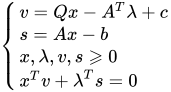
with v the Lagrange multipliers on the non-negativity constraints, λ the multipliers on the inequality constraints, and s the slack variables for the inequality constraints. The fourth condition derives from the complementarity of each group of variables (x, s) with its set of KKT vectors (optimal Lagrange multipliers) being (v, λ). In that case,

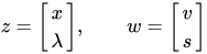
If the non-negativity constraint on the x is relaxed, the dimensionality of the LCP problem can be reduced to the number of the inequalities, as long as Q is non-singular (which is guaranteed if it is positive definite). The multipliers v are no longer present, and the first KKT conditions can be rewritten as:

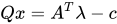
or:

pre-multiplying the two sides by A and subtracting b we obtain:

The left side, due to the second KKT condition, is s. Substituting and reordering:

Calling now

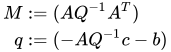
we have an LCP, due to the relation of complementarity between the slack variables s and their Lagrange multipliers λ. Once we solve it, we may obtain the value of x from λ through the first KKT condition.

Finally, it is also possible to handle additional equality constraints:

This introduces a vector of Lagrange multipliers μ, with the same dimension as .

It is easy to verify that the M and Q for the LCP system are now expressed as:

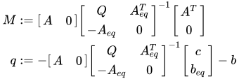
From λ we can now recover the values of both x and the Lagrange multiplier of equalities μ:

In fact, most QP solvers work on the LCP formulation, including the interior point method, principal / complementarity pivoting, and active set methods. LCP problems can be solved also by the criss-cross algorithm, conversely, for linear complementarity problems, the criss-cross algorithm terminates finitely only if the matrix is a sufficient matrix. A sufficient matrix is a generalization both of a positive-definite matrix and of a P-matrix, whose principal minors are each positive. Such LCPs can be solved when they are formulated abstractly using oriented-matroid theory.