Encyclopedia

Jacobi eigenvalue algorithm

Numerical linear algebra algorithm

Wikipedia contributorsAdapted for Fathomly · View authors

11 min read
Source updated January 6, 2026

In numerical linear algebra, the Jacobi eigenvalue algorithm is an iterative method for the calculation of the eigenvalues and eigenvectors of a real symmetric matrix (a process known as diagonalization). It is named after Carl Gustav Jacob Jacobi, who first proposed the method in 1846, but it only became widely used in the 1950s with the advent of computers.

This algorithm is inherently a dense matrix algorithm: it draws little or no advantage from being applied to a sparse matrix, and it will destroy sparseness by creating fill-in. Similarly, it will not preserve structures such as being banded of the matrix on which it operates.

01Description

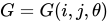
Let $S$ be a symmetric matrix, and $G=G(i,j,\theta )$ be a Givens rotation matrix. Then:

$S'=G^{\top }SG\,$

is symmetric and similar to $S$ .

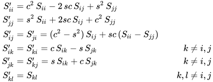
Furthermore, $S^{\prime }$ has entries:

${\begin{aligned}S'_{ii}&=c^{2}\,S_{ii}-2\,sc\,S_{ij}+s^{2}\,S_{jj}\\S'_{jj}&=s^{2}\,S_{ii}+2sc\,S_{ij}+c^{2}\,S_{jj}\\S'_{ij}&=S'_{ji}=(c^{2}-s^{2})\,S_{ij}+sc\,(S_{ii}-S_{jj})\\S'_{ik}&=S'_{ki}=c\,S_{ik}-s\,S_{jk}&k\neq i,j\\S'_{jk}&=S'_{kj}=s\,S_{ik}+c\,S_{jk}&k\neq i,j\\S'_{kl}&=S_{kl}&k,l\neq i,j\end{aligned}}$

where $s=\sin(\theta )$ and $c=\cos(\theta )$ .

Since $G$ is orthogonal, $S$ and $S^{\prime }$ have the same Frobenius norm $||\cdot ||_{F}$ (the square-root sum of squares of all components), however we can choose $\theta$ such that $S_{ij}^{\prime }=0$ , in which case $S^{\prime }$ has a larger sum of squares on the diagonal:

$S'_{ij}=\cos(2\theta )S_{ij}+{\tfrac {1}{2}}\sin(2\theta )(S_{ii}-S_{jj})$

Set this equal to 0, and rearrange:

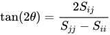
$\tan(2\theta )={\frac {2S_{ij}}{S_{jj}-S_{ii}}}$

if $S_{jj}=S_{ii}$

$\theta ={\frac {\pi }{4}}$

In order to optimize this effect, S_ij should be the off-diagonal element with the largest absolute value, called the pivot.

The Jacobi eigenvalue method repeatedly performs rotations until the matrix becomes almost diagonal. Then the elements in the diagonal are approximations of the (real) eigenvalues of S.

02Convergence

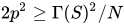
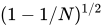
If $p=S_{kl}$ is a pivot element, then by definition $|S_{ij}|\leq |p|$ for $1\leq i,j\leq n,i\neq j$ . Let $\Gamma (S)^{2}$ denote the sum of squares of all off-diagonal entries of $S$ . Since $S$ has exactly $2N:=n(n-1)$ off-diagonal elements, we have $p^{2}\leq \Gamma (S)^{2}\leq 2Np^{2}$ or $2p^{2}\geq \Gamma (S)^{2}/N$ . Now $\Gamma (S^{J})^{2}=\Gamma (S)^{2}-2p^{2}$ . This implies $\Gamma (S^{J})^{2}\leq (1-1/N)\Gamma (S)^{2}$ or $\Gamma (S^{J})\leq (1-1/N)^{1/2}\Gamma (S)$ ; that is, the sequence of Jacobi rotations converges at least linearly by a factor $(1-1/N)^{1/2}$ to a diagonal matrix.

A number of $N$ Jacobi rotations is called a sweep; let $S^{\sigma }$ denote the result. The previous estimate yields

$\Gamma (S^{\sigma })\leq \left(1-{\frac {1}{N}}\right)^{N/2}\Gamma (S)$ ;

that is, the sequence of sweeps converges at least linearly with a factor ≈ $e^{1/2}$ .

However the following result of Schönhage yields locally quadratic convergence. To this end let S have m distinct eigenvalues $\lambda _{1},...,\lambda _{m}$ with multiplicities $\nu _{1},...,\nu _{m}$ and let d > 0 be the smallest distance of two different eigenvalues. Let us call a number of

$N_{S}:={\frac {n(n-1)}{2}}-\sum _{\mu =1}^{m}{\frac {1}{2}}\nu _{\mu }(\nu _{\mu }-1)\leq N$

Jacobi rotations a Schönhage-sweep. If $S^{s}$ denotes the result then

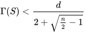
$\Gamma (S^{s})\leq {\sqrt {{\frac {n}{2}}-1}}\left({\frac {\gamma ^{2}}{d-2\gamma }}\right),\quad \gamma :=\Gamma (S)$ .

Thus convergence becomes quadratic as soon as $\Gamma (S)<{\frac {d}{2+{\sqrt {{\frac {n}{2}}-1}}}}$

03Cost

Each Givens rotation can be done in $O(n)$ steps when the pivot element p is known. However the search for p requires inspection of all N ≈ ⁠1/2⁠ n² off-diagonal elements, which means this search dominates the overall complexity and pushes the computational complexity of a sweep in the classical Jacobi algorithm to $O(n^{4})$ . Competing algorithms attain $O(n^{3})$ complexity for a full diagonalisation.

Caching row maximums

We can reduce the complexity of finding the pivot element from O(N) to O(n) if we introduce an additional index array $m_{1},\,\dots \,,\,m_{n-1}$ with the property that $m_{i}$ is the index of the largest element in row i, (i = 1, ..., n − 1) of the current S. Then the indices of the pivot (k, l) must be one of the pairs $(i,m_{i})$ . Also the updating of the index array can be done in O(n) average-case complexity: First, the maximum entry in the updated rows k and l can be found in O(n) steps. In the other rows i, only the entries in columns k and l change. Looping over these rows, if $m_{i}$ is neither k nor l, it suffices to compare the old maximum at $m_{i}$ to the new entries and update $m_{i}$ if necessary. If $m_{i}$ should be equal to k or l and the corresponding entry decreased during the update, the maximum over row i has to be found from scratch in O(n) complexity. However, this will happen on average only once per rotation. Thus, each rotation has O(n) and one sweep O(n³) average-case complexity, which is equivalent to one matrix multiplication. Additionally the $m_{i}$ must be initialized before the process starts, which can be done in n² steps.

Typically the Jacobi method converges within numerical precision after a small number of sweeps. Note that multiple eigenvalues reduce the number of iterations since $N_{S}<N$ .

Cyclic and parallel Jacobi

An alternative approach is to forego the search entirely, and simply have each sweep pivot every off-diagonal element once, in some predetermined order. It has been shown that this cyclic Jacobi attains quadratic convergence, just like the classical Jacobi.

The opportunity for parallelisation that is particular to Jacobi is based on combining cyclic Jacobi with the observation that Givens rotations for disjoint sets of indices commute, so that several can be applied in parallel. Concretely, if $G_{1}$ pivots between indices $i_{1},j_{1}$ and $G_{2}$ pivots between indices $i_{2},j_{2}$ , then from $\{i_{1},j_{1}\}\cap \{i_{2},j_{2}\}=\varnothing$ follows $G_{1}G_{2}=G_{2}G_{1}$ because in computing $G_{1}G_{2}A$ or $G_{2}G_{1}A$ the $G_{1}$ rotation only needs to access rows $i_{1},j_{1}$ and the $G_{2}$ rotation only needs to access rows $i_{2},j_{2}$ . Two processors can perform both rotations in parallel, because no matrix element is accessed for both.

Partitioning the set of index pairs of a sweep into classes that are pairwise disjoint is equivalent to partitioning the edge set of a complete graph into matchings, which is the same thing as edge colouring it; each colour class then becomes a round within the sweep. The minimal number of rounds is the chromatic index of the complete graph, and equals $n$ for odd $n$ but $n-1$ for even $n$ . A simple rule for odd $n$ is to handle the pairs $\{i_{1},j_{1}\}$ and $\{i_{2},j_{2}\}$ in the same round if $i_{1}+j_{1}\equiv i_{2}+j_{2}\textstyle {\pmod {n}}$ . For even $n$ one may create $n-1$ rounds $k=0,1,\dotsc ,n-2$ where a pair $\{i,j\}$ for $1\leqslant i<j\leqslant n-1$ goes into round $(i+j){\bmod {(}}n-1)$ and additionally a pair $\{i,n\}$ for $1\leqslant i\leqslant n-1$ goes into round $2i{\bmod {(}}n-1)$ . This brings the time complexity of a sweep down from $O(n^{3})$ to $O(n^{2})$ , if $n/2$ processors are available.

A round would consist of each processor first calculating $(c,s)$ for its rotation, and then applying the rotation from the left (rotating between rows). Next, the processors synchronise before applying the transpose rotation from the right (rotating between columns), and finally synchronising again. A matrix element may be accessed by two processors during a round, but not by both during the same half of this round.

Further parallelisation is possible by dividing the work for a single rotation between several processors, but that might be getting too fine-grained to be practical.

04Algorithm

The following algorithm is a description of the Jacobi method in math-like notation. It calculates a vector e which contains the eigenvalues and a matrix E which contains the corresponding eigenvectors; that is, $e_{i}$ is an eigenvalue and the column $E_{i}$ an orthonormal eigenvector for $e_{i}$ , i = 1, ..., n.

procedure jacobi(S ∈ R^n×n; out e ∈ Rⁿ; out E ∈ R^n×n) var i, k, l, m, state ∈ N s, c, t, p, y, d, r ∈ R ind ∈ Nⁿ changed ∈ Lⁿ function maxind(k ∈ N) ∈ N ! index of largest off-diagonal element in row k m := k+1 for i := k+2 to n do if │S_ki│ > │S_km│ then m := i endif endfor return m endfunc procedure update(k ∈ N; t ∈ R) ! update e_k and its status y := e_k; e_k := y+t if changed_k and (y=e_k) then changed_k := false; state := state−1 elsif (not changed_k) and (y≠e_k) then changed_k := true; state := state+1 endif endproc procedure rotate(k,l,i,j ∈ N) ! perform rotation of S_ij, S_kl ┌ ┐ ┌ ┐┌ ┐ │S_kl│ │c −s││S_kl│ │ │ := │ ││ │ │S_ij│ │s c││S_ij│ └ ┘ └ ┘└ ┘ endproc ! init e, E, and arrays ind, changed E := I; state := n for k := 1 to n do ind_k := maxind(k); e_k := S_kk; changed_k := true endfor while state≠0 do ! next rotation m := 1 ! find index (k,l) of pivot p for k := 2 to n−1 do if │S_{k ind_k}│ > │S_{m ind_m}│ then m := k endif endfor k := m; l := ind_m; p := S_kl ! calculate c = cos φ, s = sin φ y := (e_l−e_k)/2; d := │y│+√(p²+y²) r := √(p²+d²); c := d/r; s := p/r; t := p²/d if y<0 then s := −s; t := −t endif S_kl := 0.0; update(k,−t); update(l,t) ! rotate rows and columns k and l for i := 1 to k−1 do rotate(i,k,i,l) endfor for i := k+1 to l−1 do rotate(k,i,i,l) endfor for i := l+1 to n do rotate(k,i,l,i) endfor ! rotate eigenvectors for i := 1 to n do ┌ ┐ ┌ ┐┌ ┐ │E_ik│ │c −s││E_ik│ │ │ := │ ││ │ │E_il│ │s c││E_il│ └ ┘ └ ┘└ ┘ endfor ! update all potentially changed ind_i for i := 1 to n do ind_i := maxind(i) endfor loop endproc

Notes

1. The logical array changed holds the status of each eigenvalue. If the numerical value of $e_{k}$ or $e_{l}$ changes during an iteration, the corresponding component of changed is set to true, otherwise to false. The integer state counts the number of components of changed which have the value true. Iteration stops as soon as state = 0. This means that none of the approximations $e_{1},\,...\,,e_{n}$ has recently changed its value and thus it is not very likely that this will happen if iteration continues. Here it is assumed that floating point operations are optimally rounded to the nearest floating point number.

2. The upper triangle of the matrix S is destroyed while the lower triangle and the diagonal are unchanged. Thus it is possible to restore S if necessary according to

for k := 1 to n−1 do ! restore matrix S for l := k+1 to n do S_kl := S_lk endfor endfor

3. The eigenvalues are not necessarily in descending order. This can be achieved by a simple sorting algorithm.

for k := 1 to n−1 do m := k for l := k+1 to n do if e_l > e_m then m := l endif endfor if k ≠ m then swap e_m,e_k swap E_m,E_k endif endfor

4. The algorithm is written using matrix notation (1 based arrays instead of 0 based).

5. When implementing the algorithm, the part specified using matrix notation must be performed simultaneously.

6. This implementation does not correctly account for the case in which one dimension is an independent subspace. For example, if given a diagonal matrix, the above implementation will never terminate, as none of the eigenvalues will change. Hence, in real implementations, extra logic must be added to account for this case.

Example

Let $S={\begin{pmatrix}4&-30&60&-35\\-30&300&-675&420\\60&-675&1620&-1050\\-35&420&-1050&700\end{pmatrix}}$

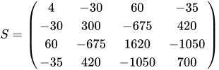
Then jacobi produces the following eigenvalues and eigenvectors after 3 sweeps (19 iterations) :

$e_{1}=2585.25381092892231$

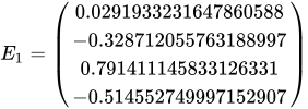
$E_{1}={\begin{pmatrix}0.0291933231647860588\\-0.328712055763188997\\0.791411145833126331\\-0.514552749997152907\end{pmatrix}}$

$e_{2}=37.1014913651276582$

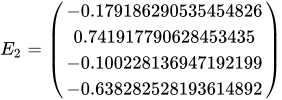
$E_{2}={\begin{pmatrix}-0.179186290535454826\\0.741917790628453435\\-0.100228136947192199\\-0.638282528193614892\end{pmatrix}}$

$e_{3}=1.4780548447781369$

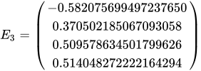
$E_{3}={\begin{pmatrix}-0.582075699497237650\\0.370502185067093058\\0.509578634501799626\\0.514048272222164294\end{pmatrix}}$

$e_{4}=0.1666428611718905$

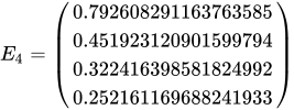
$E_{4}={\begin{pmatrix}0.792608291163763585\\0.451923120901599794\\0.322416398581824992\\0.252161169688241933\end{pmatrix}}$

05Applications for real symmetric matrices

When the eigenvalues (and eigenvectors) of a symmetric matrix are known, the following values are easily calculated.

Singular values: The singular values of a (square) matrix $A$ are the square roots of the (non-negative) eigenvalues of $A^{T}A$ . In case of a symmetric matrix $S$ we have of $S^{T}S=S^{2}$ , hence the singular values of $S$ are the absolute values of the eigenvalues of $S$ .

2-norm and spectral radius: The 2-norm of a matrix A is the norm based on the Euclidean vectornorm; that is, the largest value $\|Ax\|_{2}$ when x runs through all vectors with $\|x\|_{2}=1$ . It is the largest singular value of $A$ . In case of a symmetric matrix it is the largest absolute value of its eigenvectors and thus equal to its spectral radius.

Condition number: The condition number of a nonsingular matrix $A$ is defined as ${\mbox{cond}}(A)=\|A\|_{2}\|A^{-1}\|_{2}$ . In case of a symmetric matrix it is the absolute value of the quotient of the largest and smallest eigenvalue. Matrices with large condition numbers can cause numerically unstable results: small perturbation can result in large errors. Hilbert matrices are the most famous ill-conditioned matrices. For example, the fourth-order Hilbert matrix has a condition of 15514, while for order 8 it is 2.7 × 10⁸.

Rank: A matrix $A$ has rank $r$ if it has $r$ columns that are linearly independent while the remaining columns are linearly dependent on these. Equivalently, $r$ is the dimension of the range of $A$ . Furthermore it is the number of nonzero singular values.; In case of a symmetric matrix r is the number of nonzero eigenvalues. Unfortunately because of rounding errors numerical approximations of zero eigenvalues may not be zero (it may also happen that a numerical approximation is zero while the true value is not). Thus one can only calculate the numerical rank by making a decision which of the eigenvalues are close enough to zero.

Pseudo-inverse: The pseudo inverse of a matrix $A$ is the unique matrix $X=A^{+}$ for which $AX$ and $XA$ are symmetric and for which $AXA=A,XAX=X$ holds. If $A$ is nonsingular, then $A^{+}=A^{-1}$ .; When procedure jacobi (S, e, E) is called, then the relation $S=E^{T}{\mbox{Diag}}(e)E$ holds where Diag(e) denotes the diagonal matrix with vector e on the diagonal. Let $e^{+}$ denote the vector where $e_{i}$ is replaced by $1/e_{i}$ if $e_{i}\leq 0$ and by 0 if $e_{i}$ is (numerically close to) zero. Since matrix E is orthogonal, it follows that the pseudo-inverse of S is given by $S^{+}=E^{T}{\mbox{Diag}}(e^{+})E$ .

Least squares solution: If matrix $A$ does not have full rank, there may not be a solution of the linear system $Ax=b$ . However one can look for a vector x for which $\|Ax-b\|_{2}$ is minimal. The solution is $x=A^{+}b$ . In case of a symmetric matrix S as before, one has $x=S^{+}b=E^{T}{\mbox{Diag}}(e^{+})Eb$ .

Matrix exponential: From $S=E^{T}{\mbox{Diag}}(e)E$ one finds $\exp S=E^{T}{\mbox{Diag}}(\exp e)E$ where exp $e$ is the vector where $e_{i}$ is replaced by $\exp e_{i}$ . In the same way, $f(S)$ can be calculated in an obvious way for any (analytic) function $f$ .

Linear differential equations: The differential equation $x'=Ax,x(0)=a$ has the solution $x(t)=\exp(tA)$ . For a symmetric matrix $S$ , it follows that $x(t)=E^{T}{\mbox{Diag}}(\exp te)Ea$ . If $a=\sum _{i=1}^{n}a_{i}E_{i}$ is the expansion of $a$ by the eigenvectors of $S$ , then $x(t)=\sum _{i=1}^{n}a_{i}\exp(te_{i})E_{i}$ .; Let $W^{s}$ be the vector space spanned by the eigenvectors of $S$ which correspond to a negative eigenvalue and $W^{u}$ analogously for the positive eigenvalues. If $a\in W^{s}$ then ${\mbox{lim}}_{t\rightarrow \infty }x(t)=0$ ; that is, the equilibrium point 0 is attractive to $x(t)$ . If $a\in W^{u}$ then ${\mbox{lim}}_{t\rightarrow \infty }x(t)=\infty$ ; that is, 0 is repulsive to $x(t)$ . $W^{s}$ and $W^{u}$ are called stable and unstable manifolds for $S$ . If $a$ has components in both manifolds, then one component is attracted and one component is repelled. Hence $x(t)$ approaches $W^{u}$ as $t\to \infty$ .

06Julia implementation

The following code is a straight-forward implementation of the mathematical description of the Jacobi eigenvalue algorithm in the Julia programming language.

using LinearAlgebra, Test function find_pivot(Sprime) n = size(Sprime,1) pivot_i = pivot_j = 0 pivot = 0.0 for j = 1:n for i = 1:(j-1) if abs(Sprime[i,j]) > pivot pivot_i = i pivot_j = j pivot = abs(Sprime[i,j]) end end end return (pivot_i, pivot_j, pivot) end # in practice one should not instantiate explicitly the Givens rotation matrix function givens_rotation_matrix(n,i,j,θ) G = Matrix{Float64}(I,(n,n)) G[i,i] = G[j,j] = cos(θ) G[i,j] = sin(θ) G[j,i] = -sin(θ) return G end # S is a symmetric n by n matrix n = 4 sqrtS = randn(n,n); S = sqrtS*sqrtS'; # the largest allowed off-diagonal element of U' * S * U # where U are the eigenvectors tol = 1e-14 Sprime = copy(S) U = Matrix{Float64}(I,(n,n)) while true (pivot_i, pivot_j, pivot) = find_pivot(Sprime) if pivot < tol break end θ = atan(2*Sprime[pivot_i,pivot_j]/(Sprime[pivot_j,pivot_j] - Sprime[pivot_i,pivot_i] )) / 2 G = givens_rotation_matrix(n,pivot_i,pivot_j,θ) # update Sprime and U Sprime .= G'*Sprime*G U .= U * G end # Sprime is now (almost) a diagonal matrix # extract eigenvalues λ = diag(Sprime) # sort eigenvalues (and corresponding eigenvectors U) by increasing values i = sortperm(λ) λ = λ[i] U = U[:,i] # S should be equal to U * diagm(λ) * U' @test S ≈ U * diagm(λ) * U'

07Generalizations

The Jacobi Method has been generalized to complex Hermitian matrices, general nonsymmetric real and complex matrices as well as block matrices.

Since singular values of a real matrix are the square roots of the eigenvalues of the symmetric matrix $S=A^{T}A$ it can also be used for the calculation of these values. For this case, the method is modified in such a way that S must not be explicitly calculated which reduces the danger of round-off errors. Note that $JSJ^{T}=JA^{T}AJ^{T}=JA^{T}J^{T}JAJ^{T}=B^{T}B$ with $B\,:=JAJ^{T}$ .

Watch videos about Jacobi eigenvalue algorithmExplainers and documentaries on YouTube (opens in a new tab)

Sources and credits

This article is adapted from the Wikipedia article “Jacobi eigenvalue algorithm”, written by its contributors and licensed under CC BY-SA 4.0. Fathomly has changed the layout, removed citation markers, navigation and maintenance notices, and adjusted punctuation. This adapted version is shared under the same license. For references, see the original article.

Fathomly is not affiliated with or endorsed by the Wikimedia Foundation. Spotted a problem? Tell us.