Encyclopedia

Inverse transform sampling

Basic method for pseudo-random number sampling

Wikipedia contributorsAdapted for Fathomly · View authors

5 min read
Source updated December 29, 2025

Image credit is listed at the end of this article.

Inverse transform sampling (also known as inversion sampling, the inverse probability integral transform, the inverse transformation method, or the Smirnov transform) is a basic method for pseudo-random number sampling, i.e., for generating sample numbers at random from any probability distribution given its cumulative distribution function.

Inverse transformation sampling takes uniform samples of a number $u$ between 0 and 1, interpreted as a probability, and then returns the smallest number $x\in \mathbb {R}$ such that $F(x)\geq u$ for the cumulative distribution function $F$ of a random variable. For example, imagine that $F$ is the standard normal distribution with mean zero and standard deviation one. The table below shows samples taken from the uniform distribution and their representation on the standard normal distribution.

Transformation from uniform sample to normal
$u$	$F^{-1}(u)$
.5	0
.975	1.95996
.995	2.5758
.999999	4.75342
1-2⁻⁵²	8.12589

We are randomly choosing a proportion of the area under the curve and returning the number in the domain such that exactly this proportion of the area occurs to the left of that number. Intuitively, we are unlikely to choose a number in the far end of tails because there is very little area in them which would require choosing a number very close to zero or one.

Computationally, this method involves computing the quantile function of the distribution, in other words, computing the cumulative distribution function (CDF) of the distribution (which maps a number in the domain to a probability between 0 and 1) and then inverting that function. This is the source of the term "inverse" or "inversion" in most of the names for this method. Note that for a discrete distribution, computing the CDF is not in general too difficult: we simply add up the individual probabilities for the various points of the distribution. For a continuous distribution, however, we need to integrate the probability density function (PDF) of the distribution, which is impossible to do analytically for most distributions (including the normal distribution). As a result, this method may be computationally inefficient for many distributions and other methods are preferred; however, it is a useful method for building more generally applicable samplers such as those based on rejection sampling.

For the normal distribution, the lack of an analytical expression for the corresponding quantile function means that other methods (e.g. the Box-Muller transform) may be preferred computationally. It is often the case that, even for simple distributions, the inverse transform sampling method can be improved on: see, for example, the ziggurat algorithm and rejection sampling. On the other hand, it is possible to approximate the quantile function of the normal distribution extremely accurately using moderate-degree polynomials, and in fact the method of doing this is fast enough that inversion sampling is now the default method for sampling from a normal distribution in the statistical package R.

01Formal statement

For any random variable $X$ on $\mathbb {R}$ , the random variable $F_{X}^{-1}(U)$ has the same distribution as $X$ , where $F_{X}^{-1}$ is the generalized inverse of the cumulative distribution function $F_{X}$ of $X$ and $U$ is uniform on $[0,1]$ .

For continuous random variables, the inverse probability integral transform is indeed the inverse of the probability integral transform, which states that for a continuous random variable $X$ with cumulative distribution function $F_{X}$ , the random variable $U=F_{X}(X)$ is uniform on $[0,1]$ .

Graph of the inversion technique from to . On the bottom right we see the regular function and in the top left its inversion.

02Intuition

From $U\sim \mathrm {Unif} [0,1]$ , we want to generate $X$ with CDF $F_{X}(x).$ We assume $F_{X}(x)$ to be a continuous, strictly increasing function, which provides good intuition.

We want to see if we can find some strictly monotone transformation $T:[0,1]\mapsto \mathbb {R}$ , such that $T(U){\overset {d}{=}}X$ . We will have

$F_{X}(x)=\Pr(X\leq x)=\Pr(T(U)\leq x)=\Pr(U\leq T^{-1}(x))=T^{-1}(x),{\text{ for }}x\in \mathbb {R} ,$

where the last step used that $\Pr(U\leq y)=y$ when $U$ is uniform on $[0,1]$ .

So we got $F_{X}$ to be the inverse function of $T$ , or, equivalently $T(u)=F_{X}^{-1}(u),u\in [0,1].$

Therefore, we can generate $X$ from $F_{X}^{-1}(U).$

03The method

The problem that the inverse transform sampling method solves is as follows:

Let $X$ be a random variable whose distribution can be described by the cumulative distribution function $F_{X}$ .
We want to generate values of $X$ which are distributed according to this distribution.

The inverse transform sampling method works as follows:

Generate a random number $u$ from the standard uniform distribution in the interval $[0,1]$ , i.e. from $U\sim \mathrm {Unif} [0,1].$
Find the generalized inverse of the desired CDF, i.e. $F_{X}^{-1}(u)$ .
Compute $X'(u)=F_{X}^{-1}(u)$ . The computed random variable $X'(U)$ has distribution $F_{X}$ and thereby the same law as $X$ .

Expressed differently, given a cumulative distribution function $F_{X}$ and a uniform variable $U\in [0,1]$ , the random variable $X=F_{X}^{-1}(U)$ has the distribution $F_{X}$ .

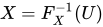
In the continuous case, a treatment of such inverse functions as objects satisfying differential equations can be given. Some such differential equations admit explicit power series solutions, despite their non-linearity.

04Examples

As an example, suppose we have a random variable $U\sim \mathrm {Unif} (0,1)$ and a cumulative distribution function

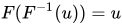
${\begin{aligned}F(x)=1-\exp(-{\sqrt {x}})\end{aligned}}$

In order to perform an inversion we want to solve for $F(F^{-1}(u))=u$

${\begin{aligned}F(F^{-1}(u))&=u\\1-\exp \left(-{\sqrt {F^{-1}(u)}}\right)&=u\\F^{-1}(u)&=(-\log(1-u))^{2}\\&=(\log(1-u))^{2}\end{aligned}}$

From here we would perform steps one, two and three.

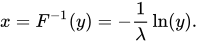
As another example, we use the exponential distribution with $F_{X}(x)=1-e^{-\lambda x}$ for x ≥ 0 (and 0 otherwise). By solving y=F(x) we obtain the inverse function

$x=F^{-1}(y)=-{\frac {1}{\lambda }}\ln(1-y).$

It means that if we draw some $y_{0}$ from a $U\sim \mathrm {Unif} (0,1)$ and compute $x_{0}=F_{X}^{-1}(y_{0})=-{\frac {1}{\lambda }}\ln(1-y_{0}),$ This $x_{0}$ has exponential distribution.

The idea is illustrated in the following graph:

Note that the distribution does not change if we start with 1-y instead of y. For computational purposes, it therefore suffices to generate random numbers y in [0, 1] and then simply calculate

$x=F^{-1}(y)=-{\frac {1}{\lambda }}\ln(y).$

05Proof of correctness

Let $F$ be a cumulative distribution function, and let $F^{-1}$ be its generalized inverse function (using the infimum because CDFs are weakly monotonic and right-continuous):

$F^{-1}(u)=\inf \;\{x\mid F(x)\geq u\}\qquad (0<u<1).$

Claim: If $U$ is a uniform random variable on $[0,1]$ then $F^{-1}(U)$ has $F$ as its CDF.

Proof:

${\begin{aligned}&\Pr(F^{-1}(U)\leq x)\\&{}=\Pr(U\leq F(x))\quad &(F{\text{ is right-continuous, so }}\{u:F^{-1}(u)\leq x\}=\{u:u\leq F(x)\})\\&{}=F(x)\quad &({\text{because }}\Pr(U\leq u)=u,{\text{ when }}U{\text{ is uniform on }}[0,1])\\\end{aligned}}$

An animation of how inverse transform sampling generates normally distributed random values from uniformly distributed random values

06Truncated distribution

Inverse transform sampling can be simply extended to cases of truncated distributions on the interval $(a,b]$ without the cost of rejection sampling: the same algorithm can be followed, but instead of generating a random number $u$ uniformly distributed between 0 and 1, generate $u$ uniformly distributed between $F(a)$ and $F(b)$ , and then again take $F^{-1}(u)$ .

07Reduction of the number of inversions

In order to obtain a large number of samples, one needs to perform the same number of inversions of the distribution. One possible way to reduce the number of inversions while obtaining a large number of samples is the application of the so-called Stochastic Collocation Monte Carlo sampler (SCMC sampler) within a polynomial chaos expansion framework. This allows us to generate any number of Monte Carlo samples with only a few inversions of the original distribution with independent samples of a variable for which the inversions are analytically available, for example the standard normal variable.

08Software implementations

There are software implementations available for applying the inverse sampling method by using numerical approximations of the inverse in the case that it is not available in closed form. For example, an approximation of the inverse can be computed if the user provides some information about the distributions such as the PDF or the CDF.

C library UNU.RAN
R library Runuran
Python subpackage sampling in scipy.stats

Watch videos about Inverse transform samplingExplainers and documentaries on YouTube (opens in a new tab)

Sources and credits

This article is adapted from the Wikipedia article “Inverse transform sampling”, written by its contributors and licensed under CC BY-SA 4.0. Fathomly has changed the layout, removed citation markers, navigation and maintenance notices, and adjusted punctuation. This adapted version is shared under the same license. For references, see the original article.

Images, from Wikimedia Commons:

Inverse transform sampling.png by Olivier Ricou, CC BY-SA 3.0
InverseFunc.png by Steve Bronder, CC BY-SA 4.0
Generalized inversion method.svg by Ta2o, CC BY-SA 4.0
Inverse Transform Sampling Example.gif by Davidjessop, CC BY-SA 4.0
Inverse transformation method for exponential distribution.jpg by LarsWinterfeld, CC BY-SA 4.0

Fathomly is not affiliated with or endorsed by the Wikimedia Foundation. Spotted a problem? Tell us.