Encyclopedia

Interval estimation

Interval bounded by an upper and a lower limit statistics

Wikipedia contributorsAdapted for Fathomly · View authors

7 min read
Source updated April 15, 2026

In statistics, interval estimation is the use of sample data to estimate an interval of possible values of a (sample) parameter of interest. This is in contrast to point estimation, which gives a single value.

The most prevalent forms of interval estimation are confidence intervals (a frequentist method) and credible intervals (a Bayesian method). Less common forms include likelihood intervals, fiducial intervals, tolerance intervals, and prediction intervals. For a non-statistical method, interval estimates can be deduced from fuzzy logic.

01Types

Confidence intervals

Confidence intervals are used to estimate the parameter of interest from a sampled data set, commonly the mean or standard deviation. A confidence interval states there is a 100γ% confidence that the parameter of interest is within a lower and upper bound. A common misconception of confidence intervals is 100γ% of the data set fits within or above/below the bounds, this is referred to as a tolerance interval, which is discussed below.

There are multiple methods used to build a confidence interval, the correct choice depends on the data being analyzed. For a normal distribution with a known variance, one uses the z-table to create an interval where a confidence level of 100γ% can be obtained centered around the sample mean from a data set of n measurements. For a binomial distribution, confidence intervals can be approximated using the Wald approximate method, Jeffreys interval, and Clopper-Pearson interval. The Jeffrey method can also be used to approximate intervals for a Poisson distribution. If the underlying distribution is unknown, one can utilize bootstrapping to create bounds about the median of the data set.

Credible intervals

As opposed to a confidence interval, a credible interval requires a prior assumption, modifying the assumption utilizing a Bayes factor, and determining a posterior distribution. Utilizing the posterior distribution, one can determine a 100γ% probability the parameter of interest is included, as opposed to the confidence interval where one can be 100γ% confident that an estimate is included within an interval.

${\text{Posterior}}\ \propto \ {\text{Likelihood}}\times {\text{Prior}}$

While a prior assumption is helpful towards providing more data towards building an interval, it removes the objectivity of a confidence interval. A prior will be used to inform a posterior, if unchallenged this prior can lead to incorrect predictions.

The credible interval's bounds are variable, unlike the confidence interval. There are multiple methods to determine where the correct upper and lower limits should be located. Common techniques to adjust the bounds of the interval include highest posterior density interval (HPDI), equal-tailed interval, or choosing the center the interval around the mean.

Less common forms

Likelihood-based

Utilizes the principles of a likelihood function to estimate the parameter of interest. Utilizing the likelihood-based method, confidence intervals can be found for exponential, Weibull, and lognormal means. Additionally, likelihood-based approaches can give confidence intervals for the standard deviation. It is also possible to create a prediction interval by combining the likelihood function and the future random variable.

Fiducial

Fiducial inference utilizes a data set, carefully removes the noise and recovers a distribution estimator, generalized fiducial distribution (GFD). Without the use of Bayes' theorem, there is no assumption of a prior, much like confidence intervals. Fiducial inference is a less common form of statistical inference. The founder, R.A. Fisher, who had been developing inverse probability methods, had his own questions about the validity of the process. While fiducial inference was developed in the early twentieth century, the late twentieth century believed that the method was inferior to the frequentist and Bayesian approaches but held an important place in historical context for statistical inference. However, modern-day approaches have generalized the fiducial interval into generalized fiducial inference (GFI), which can be used to estimate discrete and continuous data sets.

Tolerance

Tolerance intervals use collected data set population to obtain an interval, within tolerance limits, containing 100γ% values. Examples typically used to describe tolerance intervals include manufacturing. In this context, a percentage of an existing product set is evaluated to ensure that a percentage of the population is included within tolerance limits. When creating tolerance intervals, the bounds can be written in terms of an upper and lower tolerance limit, utilizing the sample mean, $\mu$ , and the sample standard deviation, s.

$(l_{b},u_{b})=\mu \pm k_{2}s$ for two-sided intervals

for two-sided intervals

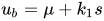
And in the case of one-sided intervals where the tolerance is required only above or below a critical value,

$l_{b}=\mu -k_{1}s$ $u_{b}=\mu +k_{1}s$

$k_{i}$ varies by distribution and the number of sides, i, in the interval estimate. In a normal distribution, $k_{2}$ can be expressed as

$k_{2}=z_{\alpha /2}{\sqrt {{\frac {\nu }{\chi _{1-\alpha ,\nu }^{2}}}\left(1+{\frac {1}{N}}\right)}}$

where $\chi _{1-\alpha ,\nu }^{2}$ is the critical value of the chi-square distribution utilizing $\nu$ degrees of freedom that is exceeded with probability $\alpha$ , and $z_{\alpha /2}$ is the critical values obtained from the normal distribution.

Prediction

A prediction interval estimates the interval containing future samples with some confidence, γ. Prediction intervals can be used for both Bayesian and frequentist contexts. These intervals are typically used in regression data sets, but prediction intervals are not used for extrapolation beyond the previous data's experimentally controlled parameters.

Fuzzy logic

Fuzzy logic is used to handle decision-making in a non-binary fashion for artificial intelligence, medical decisions, and other fields. In general, it takes inputs, maps them through fuzzy inference systems, and produces an output decision. This process involves fuzzification, fuzzy logic rule evaluation, and defuzzification. When looking at fuzzy logic rule evaluation, membership functions convert our non-binary input information into tangible variables. These membership functions are essential to predict the uncertainty of the system.

02One-sided vs. two-sided

Two-sided intervals estimate a parameter of interest, Θ, with a level of confidence, γ, using a lower ( $l_{b}$ ) and upper bound ( $u_{b}$ ). Examples may include estimating the average height of males in a geographic region or lengths of a particular desk made by a manufacturer. These cases tend to estimate the central value of a parameter. Typically, this is presented in a form similar to the equation below.

$P(l_{b}<\Theta <u_{b})=\gamma$

Differentiating from the two-sided interval, the one-sided interval utilizes a level of confidence, γ, to construct a minimum or maximum bound which predicts the parameter of interest to γ*100% probability. Typically, a one-sided interval is required when the estimate's minimum or maximum bound is not of interest. When concerned about the minimum predicted value of Θ, one is no longer required to find an upper bounds of the estimate, leading to a form reduced form of the two-sided.

$P(l_{b}<\Theta )=\gamma$

As a result of removing the upper bound and maintaining the confidence, the lower-bound ( $l_{b}$ ) will increase. Likewise, when concerned with finding only an upper bound of a parameter's estimate, the upper bound will decrease. A one-sided interval is a commonly found in material production's quality assurance, where an expected value of a material's strength, Θ, must be above a certain minimum value ( $l_{b}$ ) with some confidence (100γ%). In this case, the manufacturer is not concerned with producing a product that is too strong, there is no upper-bound ( $u_{b}$ ).

03Discussion

When determining the statistical significance of a parameter, it is best to understand the data and its collection methods. Before collecting data, an experiment should be planned such that the sampling error is statistical variability (a random error), as opposed to a statistical bias (a systematic error). After experimenting, a typical first step in creating interval estimates is exploratory analysis plotting using various graphical methods. From this, one can determine the distribution of samples from the data set. Producing interval boundaries with incorrect assumptions based on distribution makes a prediction faulty.

When interval estimates are reported, they should have a commonly held interpretation within and beyond the scientific community. Interval estimates derived from fuzzy logic have much more application-specific meanings.

In commonly occurring situations there should be sets of standard procedures that can be used, subject to the checking and validity of any required assumptions. This applies for both confidence intervals and credible intervals. However, in more novel situations there should be guidance on how interval estimates can be formulated. In this regard confidence intervals and credible intervals have a similar standing but there two differences. First, credible intervals can readily deal with prior information, while confidence intervals cannot. Secondly, confidence intervals are more flexible and can be used practically in more situations than credible intervals: one area where credible intervals suffer in comparison is in dealing with non-parametric models.

There should be ways of testing the performance of interval estimation procedures. This arises because many such procedures involve approximations of various kinds and there is a need to check that the actual performance of a procedure is close to what is claimed. The use of stochastic simulations makes this is straightforward in the case of confidence intervals, but it is somewhat more problematic for credible intervals where prior information needs to be taken properly into account. Checking of credible intervals can be done for situations representing no-prior-information but the check involves checking the long-run frequency properties of the procedures.

Severini (1993) discusses conditions under which credible intervals and confidence intervals will produce similar results, and also discusses both the coverage probabilities of credible intervals and the posterior probabilities associated with confidence intervals.

In decision theory, which is a common approach to and justification for Bayesian statistics, interval estimation is not of direct interest. The outcome is a decision, not an interval estimate, and thus Bayesian decision theorists use a Bayes action: they minimize expected loss of a loss function with respect to the entire posterior distribution, not a specific interval.

04Applications

Applications of confidence intervals are used to solve a variety of problems dealing with uncertainty. Katz (1975) proposes various challenges and benefits for utilizing interval estimates in legal proceedings. For use in medical research, Altmen (1990) discusses the use of confidence intervals and guidelines towards using them. In manufacturing, it is also common to find interval estimates estimating a product life, or to evaluate the tolerances of a product. Meeker and Escobar (1998) present methods to analyze reliability data under parametric and nonparametric estimation, including the prediction of future, random variables (prediction intervals).

Watch videos about Interval estimationExplainers and documentaries on YouTube (opens in a new tab)

Sources and credits

This article is adapted from the Wikipedia article “Interval estimation”, written by its contributors and licensed under CC BY-SA 4.0. Fathomly has changed the layout, removed citation markers, navigation and maintenance notices, and adjusted punctuation. This adapted version is shared under the same license. For references, see the original article.

Images, from Wikimedia Commons:

Prior, Likelihood, Posterior schematic.svg by Rbb, CC BY-SA 3.0
Confidence Interval Differentiation.png by Grw66, CC0

Fathomly is not affiliated with or endorsed by the Wikimedia Foundation. Spotted a problem? Tell us.