Encyclopedia

Image derivative

Wikipedia contributorsAdapted for Fathomly · View authors

4 min read
Source updated October 3, 2025

Image derivatives can be computed by using small convolution filters of size 2 × 2 or 3 × 3, such as the Laplacian, Sobel, Roberts and Prewitt operators. However, a larger mask will generally give a better approximation of the derivative and examples of such filters are Gaussian derivatives and Gabor filters. Sometimes high frequency noise needs to be removed and this can be incorporated in the filter so that the Gaussian kernel will act as a band pass filter. The use of Gabor filters in image processing has been motivated by some of its similarities to the perception in the human visual system.

The pixel value is computed as a convolution

$p'_{u}=\mathbf {d} \ast G$

where $\mathbf {d}$ is the derivative kernel and $G$ is the pixel values in a region of the image and $\ast$ is the operator that performs the convolution.

01Sobel derivatives

The derivative kernels, known as the Sobel operator are defined as follows, for the $u$ and $v$ directions respectively:

$p'_{u}={\begin{bmatrix}+1&+2&+1\\0&0&0\\-1&-2&-1\end{bmatrix}}*\mathbf {G} \quad {\mbox{and}}\quad p'_{v}={\begin{bmatrix}+1&0&-1\\+2&0&-2\\+1&0&-1\end{bmatrix}}*\mathbf {G}$

where $*$ here denotes the 2-dimensional convolution operation.

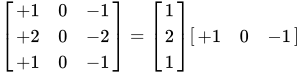
This operator is separable and can be decomposed as the products of an interpolation and a differentiation kernel, so that, $p'_{v}$ , for an example can be written as

${\begin{bmatrix}+1&0&-1\\+2&0&-2\\+1&0&-1\end{bmatrix}}={\begin{bmatrix}1\\2\\1\end{bmatrix}}{\begin{bmatrix}+1&0&-1\end{bmatrix}}$

02Farid and Simoncelli derivatives

Farid and Simoncelli propose to use a pair of kernels, one for interpolation and another for differentiation (compare to Sobel above). These kernels, of fixed sizes 5 x 5 and 7 x 7, are optimized so that the Fourier transform approximates their correct derivative relationship.

In Matlab code the so called 5-tap filter is

k = [0.030320 0.249724 0.439911 0.249724 0.030320]; d = [0.104550 0.292315 0.000000 -0.292315 -0.104550]; d2 = [0.232905 0.002668 -0.471147 0.002668 0.232905];

And the 7-tap filter is

k = [ 0.004711 0.069321 0.245410 0.361117 0.245410 0.069321 0.004711]; d = [ 0.018708 0.125376 0.193091 0.000000 -0.193091 -0.125376 -0.018708]; d2 = [ 0.055336 0.137778 -0.056554 -0.273118 -0.056554 0.137778 0.055336];

As an example the first order derivatives can be computed in the following using Matlab in order to perform the convolution

Iu = conv2(d, k, im, 'same'); % derivative vertically (wrt Y) Iv = conv2(k, d, im, 'same'); % derivative horizontally (wrt X)

It is noted that Farid and Simoncelli have derived first derivative coefficients which are more accurate compared to the ones provided above. However, the latter are consistent with the second derivative interpolator and, therefore, are better to use if both the first and second derivatives are sought. In the opposite case, when only the first derivative is desired, the optimal first derivative coefficients should be employed; more details can be found in their paper.

03Hast derivatives

Derivative filters based on arbitrary cubic splines was presented by Hast. He showed how both first and second order derivatives can be computed more correctly using cubic or trigonometric splines. Efficient derivative filters need to be of odd length so that the derivative is computed for the central pixel. However, any cubic filter is fitted over 4 sample points, giving a centre that falls between pixels. This is solved by a double filtering approach giving filters of size 7 x 7. The idea is to first filter by interpolation so that the interpolated value between pixels are obtained, whereafter the procedure is repeated using a derivative filters, where the centre value now falls on pixel centres. This can easily be proved by the associative law for convolution

$p'_{u}=\mathbf {d} \ast (\mathbf {k} \ast G)=(\mathbf {d} \ast \mathbf {k} )\ast G$

Therefore the convolution kernel for computing the derivative $\mathbf {k_{d}}$ using an interpolating kernel $\mathbf {k}$ and a derivative kernel $\mathbf {d}$ becomes

$\mathbf {k_{d}} =\mathbf {d} \ast \mathbf {k}$

Also keep in mind that convolution is commutative, so that the order of the two kernels does not matter and it is also possible to insert a second order derivative as well as a first order derivative kernel. These kernels are derived from the fact that any spline surface can be fitted over a square pixel region, compare to Bezier surfaces. Hast proves that such a surface can be performed as a separable convolution

$p(u,v)=\mathbf {u} ^{T}MGM^{T}\mathbf {v} =M^{T}\mathbf {u} \otimes \mathbf {v} ^{T}M\ast G$

where $M$ is the spline basis matrix, $\mathbf {u}$ and $\mathbf {v}$ are vectors containing the variables $u$ and $v$ , such as

$\mathbf {u} =[u^{3},u^{2},u,1]^{T}$

$\mathbf {v} =[v^{3},v^{2},v,1]^{T}$

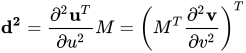
The convolution kernels can now be set to

$\mathbf {k} =\mathbf {u} ^{T}M=(M^{T}\mathbf {v} )^{T}$

$\mathbf {d} ={\frac {\partial \mathbf {u} ^{T}}{\partial u}}M=\left(M^{T}{\frac {\partial \mathbf {v} }{\partial v}}\right)^{T}$

$\mathbf {d^{2}} ={\frac {\partial ^{2}\mathbf {u} ^{T}}{\partial u^{2}}}M=\left(M^{T}{\frac {\partial ^{2}\mathbf {v} }{\partial v^{2}}}\right)^{T}$

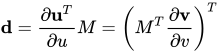
The first order derivatives at the central pixel are hence computed as

$D_{u}={\frac {\partial \mathbf {u} ^{T}}{\partial u}}M\ast \mathbf {u} ^{T}MGM^{T}\mathbf {v} \ast M^{T}\mathbf {v} =\mathbf {d} \ast \mathbf {k} \otimes (\mathbf {k} \ast \mathbf {k} )^{T}\ast G$

and

$D_{v}=\mathbf {u} ^{T}M\ast \mathbf {u} ^{T}MGM^{T}\mathbf {v} \ast M^{T}{\frac {\partial \mathbf {v} }{\partial v}}=\mathbf {k} \ast \mathbf {k} \otimes (\mathbf {d} \ast \mathbf {k} )^{T}\ast G$

Likewise, with the second order derivative kernels are

$D_{u}^{2}={\frac {\partial ^{2}\mathbf {u} ^{T}}{\partial u^{2}}}M\ast \mathbf {u} ^{T}MGM^{T}\mathbf {v} \ast M^{T}\mathbf {v} =\mathbf {d^{2}} \ast \mathbf {k} \otimes (\mathbf {k} \ast \mathbf {k} )^{T}\ast G$

and

$D_{v}^{2}=\mathbf {u} ^{T}M\ast \mathbf {u} ^{T}MGM^{T}\mathbf {v} \ast M^{T}{\frac {\partial ^{2}\mathbf {v} }{\partial v^{2}}}=\mathbf {k} \ast \mathbf {k} \otimes (\mathbf {d^{2}} \ast \mathbf {k} )^{T}\ast G$

The cubic spline filter is evaluated in its centre $u=v=0.5$ and therefore

$\mathbf {u} =\mathbf {v} =[(0.5)^{3},(0.5)^{2},0.5,1]^{T}=[0.125,0.25,0.5,1]^{T}$

Likewise the first order derivatives becomes

${\frac {\partial \mathbf {u} (0.5)}{\partial u}}={\frac {\partial \mathbf {v} (0.5)}{\partial v}}=[3\cdot (0.5)^{2},2\cdot (0.5),1,0]^{T}=[0.75,1,1,0]^{T}$

And in a similar manner the second order derivatives are

${\frac {d^{2}\mathbf {u} (0.5)}{u^{2}}}={\frac {d^{2}\mathbf {v} (0.5)}{dv^{2}}}=[6\cdot (0.5),2,0,0]^{T}=[3,2,0,0]^{T}$

Any cubic filter can be applied and used for computing the image derivates using the above equations, such as Bézier, Hermite or B-splines.

The example in below in Matlab use the Catmull-Rom spline to compute the derivatives

M = [1,-3,3,-1; -1,4,-5,2; 0,1,0,-1; 0,0,2,0] * 0.5; u = [0.125;0.25;0.5;1]; up = [0.75;1;1;0]; d = up'*M; k = u'*M; Iu = conv2(conv(d, k), conv(k, k), im,'same'); % vertical derivative (wrt Y) Iv = conv2(conv(k, k), conv(d, k), im,'same'); % horizontal derivative (wrt X)

04Other approaches

Steerable filters can be used for computing derivatives Moreover, Savitzky and Golay propose a least-squares polynomial smoothing approach, which could be used for computing derivatives and Luo et al discuss this approach in further detail. Scharr shows how to create derivative filters by minimizing the error in the Fourier domain and Jähne et al discuss in more detail the principles of filter design, including derivative filters.

Watch videos about Image derivativeExplainers and documentaries on YouTube (opens in a new tab)

Sources and credits

This article is adapted from the Wikipedia article “Image derivative”, written by its contributors and licensed under CC BY-SA 4.0. Fathomly has changed the layout, removed citation markers, navigation and maintenance notices, and adjusted punctuation. This adapted version is shared under the same license. For references, see the original article.

Fathomly is not affiliated with or endorsed by the Wikimedia Foundation. Spotted a problem? Tell us.