Hyperbolic equilibrium point
Fixed point that does not have any center manifolds

In the study of dynamical systems, a hyperbolic equilibrium point or hyperbolic fixed point is a fixed point that does not have any center manifolds. Near a hyperbolic point the orbits of a two-dimensional, non-dissipative system resemble hyperbolas. This fails to hold in general. Strogatz notes that "hyperbolic is an unfortunate name, it sounds like it should mean 'saddle point', but it has become standard." Several properties hold about a neighborhood of a hyperbolic point, notably
- A stable manifold and an unstable manifold exist,
- Shadowing occurs,
- The dynamics on the invariant set can be represented via symbolic dynamics,
- A natural measure can be defined,
- The system is structurally stable.
01Maps
If 

One example of a map whose only fixed point is hyperbolic is Arnold's cat map:
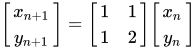
Since the eigenvalues are given by
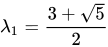
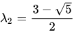
We know that the Lyapunov exponents are:
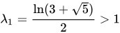
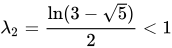
Therefore, it is a saddle point.
02Flows
Let 
The Hartman-Grobman theorem states that the orbit structure of a dynamical system in a neighbourhood of a hyperbolic equilibrium point is topologically equivalent to the orbit structure of the linearized dynamical system.
Example
Consider the nonlinear system
![{\begin{aligned}{\frac {dx}{dt}}&=y,\\[5pt]{\frac {dy}{dt}}&=-x-x^{3}-\alpha y,~\alpha \neq 0\end{aligned}}](https://wikimedia.org/api/rest_v1/media/math/render/svg/8f94314d229d84506a4f5a68d51e672d2fa3334b)
(0, 0) is the only equilibrium point. The Jacobian matrix of the linearization at the equilibrium point is
![J(0,0)=\left[{\begin{array}{rr}0&1\\-1&-\alpha \end{array}}\right].](https://wikimedia.org/api/rest_v1/media/math/render/svg/a9a02f9987490279fb5050b999d067f361ce42b3)
The eigenvalues of this matrix are 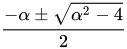
Sources and credits
This article is adapted from the Wikipedia article “Hyperbolic equilibrium point”, written by its contributors and licensed under CC BY-SA 4.0. Fathomly has changed the layout, removed citation markers, navigation and maintenance notices, and adjusted punctuation. This adapted version is shared under the same license. For references, see the original article.
Images, from Wikimedia Commons:
- Phase Portrait Sadle.svg by Podshumok This W3C-unspecified vector image was created with Inkscape ., CC BY-SA 3.0
Fathomly is not affiliated with or endorsed by the Wikimedia Foundation. Spotted a problem? Tell us.
03Comments
In the case of an infinite dimensional system, for example systems involving a time delay, the notion of the "hyperbolic part of the spectrum" refers to the above property.