Encyclopedia

Fixed-point computation

Computing the fixed point of a function

Wikipedia contributorsAdapted for Fathomly · View authors

9 min read
Source updated December 27, 2025

Fixed-point computation refers to the process of computing an exact or approximate fixed point of a given function. In its most common form, the given function $f$ satisfies the condition to the Brouwer fixed-point theorem: that is, $f$ is continuous and maps the unit d-cube to itself. The Brouwer fixed-point theorem guarantees that $f$ has a fixed point, but the proof is not constructive. Various algorithms have been devised for computing an approximate fixed point. Such algorithms are used in various tasks, such as

01Definitions

The unit interval is denoted by $E:=[0,1]$ , and the unit d-dimensional cube is denoted by $E^{d}$ . A continuous function $f$ is defined on $E^{d}$ (from $E^{d}$ to itself). Often, it is assumed that $f$ is not only continuous but also Lipschitz continuous, that is, for some constant $L$ , $|f(x)-f(y)|\leq L\cdot |x-y|$ for all $x,y$ in $E^{d}$ .

A fixed point of $f$ is a point $x$ in $E^{d}$ such that $f(x)=x$ . By the Brouwer fixed-point theorem, any continuous function from $E^{d}$ to itself has a fixed point. But for general functions, it is impossible to compute a fixed point precisely, since it can be an arbitrary real number. Fixed-point computation algorithms look for approximate fixed points. There are several criteria for an approximate fixed point. Several common criteria are:

The residual criterion: given an approximation parameter $\varepsilon >0$ , An ε-residual fixed-point of $f$ is a point $x$ in $E^{d}$ ' such that $|f(x)-x|\leq \varepsilon$ , where here $|\cdot |$ denotes the maximum norm. That is, all $d$ coordinates of the difference $f(x)-x$ should be at most ε.
The absolute criterion: given an approximation parameter $\delta >0$ , A δ-absolute fixed-point of $f$ is a point $x$ in $E^{d}$ such that $|x-x_{0}|\leq \delta$ , where $x_{0}$ is any fixed-point of $f$ .
The relative criterion: given an approximation parameter $\delta >0$ , A δ-relative fixed-point of $f$ is a point x in $E^{d}$ such that $|x-x_{0}|/|x_{0}|\leq \delta$ , where $x_{0}$ is any fixed-point of $f$ .

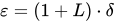
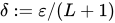
For Lipschitz-continuous functions, the absolute criterion is stronger than the residual criterion: If $f$ is Lipschitz-continuous with constant $L$ , then $|x-x_{0}|\leq \delta$ implies $|f(x)-f(x_{0})|\leq L\cdot \delta$ . Since $x_{0}$ is a fixed-point of $f$ , this implies $|f(x)-x_{0}|\leq L\cdot \delta$ , so $|f(x)-x|\leq (1+L)\cdot \delta$ . Therefore, a δ-absolute fixed-point is also an ε-residual fixed-point with $\varepsilon =(1+L)\cdot \delta$ .

The most basic step of a fixed-point computation algorithm is a value query: given any $x$ in $E^{d}$ , the algorithm is provided with an oracle ${\tilde {f}}$ to $f$ that returns the value $f(x)$ . The accuracy of the approximate fixed-point depends upon the error in the oracle ${\tilde {f}}(x)$ .

The function $f$ is accessible via evaluation queries: for any $x$ , the algorithm can evaluate $f(x)$ . The run-time complexity of an algorithm is usually given by the number of required evaluations.

02Contractive functions

A Lipschitz-continuous function with constant $L$ is called contractive if $L<1$ ; it is called weakly-contractive if $L\leq 1$ . Every contractive function satisfying Brouwer's conditions has a unique fixed point. Moreover, fixed-point computation for contractive functions is easier than for general functions.

The first algorithm for fixed-point computation was the fixed-point iteration algorithm of Banach. Banach's fixed-point theorem implies that, when fixed-point iteration is applied to a contraction mapping, the error after $t$ iterations is in $O(L^{t})$ . Therefore, the number of evaluations required for a $\delta$ -relative fixed-point is approximately $\log _{L}(\delta )=\log(\delta )/\log(L)=\log(1/\delta )/\log(1/L)$ . Sikorski and Wozniakowski showed that Banach's algorithm is optimal when the dimension is large. Specifically, when $d\geq \log(1/\delta )/\log(1/L)$ , the number of required evaluations of any algorithm for $\delta$ -relative fixed-point is larger than 50% the number of evaluations required by the iteration algorithm. Note that when $L$ approaches 1, the number of evaluations approaches infinity. No finite algorithm can compute a $\delta$ -absolute fixed point for all functions with $L=1$ .

When $L$ < 1 and d = 1, the optimal algorithm is the Fixed Point Envelope (FPE) algorithm of Sikorski and Wozniakowski. It finds a δ-relative fixed point using $O(\log(1/\delta )+\log \log(1/(1-L)))$ queries, and a δ-absolute fixed point using $O(\log(1/\delta ))$ queries. This is faster than the fixed-point iteration algorithm.

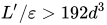
When $d>1$ but not too large, and $L\leq 1$ , the optimal algorithm is the interior-ellipsoid algorithm (based on the ellipsoid method). It finds an ε-residual fixed-point using $O(d\cdot \log(1/\varepsilon ))$ evaluations. When $L<1$ , it finds a $\delta$ -absolute fixed point using $O(d\cdot [\log(1/\delta )+\log(1/(1-L))])$ evaluations.

Shellman and Sikorski presented an algorithm called BEFix (Bisection Envelope Fixed-point) for computing an ε-residual fixed-point of a two-dimensional function with ' $L\leq 1$ , using only $2\lceil \log _{2}(1/\varepsilon )\rceil +1$ queries. They later presented an improvement called BEDFix (Bisection Envelope Deep-cut Fixed-point), with the same worst-case guarantee but better empirical performance. When $L<1$ , BEDFix can also compute a $\delta$ -absolute fixed-point using $O(\log(1/\varepsilon )+\log(1/(1-L)))$ queries.

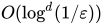
Shellman and Sikorski presented an algorithm called PFix for computing an ε-residual fixed-point of a d-dimensional function with L ≤ 1, using $O(\log ^{d}(1/\varepsilon ))$ queries. When $L$ < 1, PFix can be executed with $\varepsilon =(1-L)\cdot \delta$ , and in that case, it computes a δ-absolute fixed-point, using $O(\log ^{d}(1/[(1-L)\delta ]))$ queries. It is more efficient than the iteration algorithm when $L$ is close to 1. The algorithm is recursive: it handles a d-dimensional function by recursive calls on (d-1)-dimensional functions.

Algorithms for differentiable functions

When the function $f$ is differentiable, and the algorithm can evaluate its derivative (not only $f$ itself), the Newton method can be used and it is much faster.

03General functions: one dimension

For functions with Lipschitz constant $L$ > 1, computing a fixed-point is much harder.

For a 1-dimensional function (d = 1), a $\delta$ -absolute fixed-point can be found using $O(\log(1/\delta ))$ queries using the bisection method: start with the interval $E:=[0,1]$ ; at each iteration, let $x$ be the center of the current interval, and compute $f(x)$ ; if $f(x)>x$ then recurse on the sub-interval to the right of $x$ ; otherwise, recurse on the interval to the left of $x$ . Note that the current interval always contains a fixed point, so after $O(\log(1/\delta ))$ queries, any point in the remaining interval is a $\delta$ -absolute fixed-point of $f$ Setting $\delta :=\varepsilon /(L+1)$ , where $L$ is the Lipschitz constant, gives an ε-residual fixed-point, using $O(\log(L/\varepsilon )=\log(L)+\log(1/\varepsilon ))$ queries.

04General functions: two or more dimensions

For functions in two or more dimensions, the problem is much more challenging. Shellman and Sikorski proved that for any integers d ≥ 2 and $L$ > 1, finding a δ-absolute fixed-point of d-dimensional $L$ -Lipschitz functions might require infinitely many evaluations. The proof idea is as follows. For any integer T > 1 and any sequence of T of evaluation queries (possibly adaptive), one can construct two functions that are Lipschitz-continuous with constant $L$ , and yield the same answer to all these queries, but one of them has a unique fixed-point at (x, 0) and the other has a unique fixed-point at (x, 1). Any algorithm using T evaluations cannot differentiate between these functions, so cannot find a δ-absolute fixed-point. This is true for any finite integer T.

Several algorithms based on function evaluations have been developed for finding an ε-residual fixed-point.

Simplicial method

The first algorithm to approximate a fixed point of a general function was developed by Herbert Scarf in 1967. Scarf's algorithm finds an ε-residual fixed-point by finding a fully labeled "primitive set", in a construction similar to Sperner's lemma.

A later algorithm by Harold Kuhn used simplices and simplicial partitions instead of primitive sets.

Developing the simplicial approach further, Orin Harrison Merrill presented the restart algorithm.

Homotopy method

B. Curtis Eaves presented the homotopy method, based on the concept of homotopy.

Given a function f, for which we want to find a fixed point, the algorithm works by starting with an affine function that approximates f, and deforming it towards f while following the fixed point.

The homotopy method has been used for market equilibrium computation.

The method is further explained in a book by Michael Todd, which surveys various algorithms developed until 1976.

Other algorithms

David Gale showed that computing a fixed point of an n-dimensional function (on the unit d-dimensional cube) is equivalent to deciding who is the winner in a d-dimensional game of Hex (a game with d players, each of whom needs to connect two opposite faces of a d-cube). Given the desired accuracy ε
- Construct a Hex board of size kd, where $k>1/\varepsilon$ . Each vertex z corresponds to a point z/k in the unit n-cube.
- Compute the difference $f$ (z/k) - z/k; note that the difference is an n-vector.
- Label the vertex z by a label in 1, ..., d, denoting the largest coordinate in the difference vector.
- The resulting labeling corresponds to a possible play of the d-dimensional Hex game among d players. This game must have a winner, and Gale presents an algorithm for constructing the winning path.
- In the winning path, there must be a point in which f_i(z/k) - z/k is positive, and an adjacent point in which f_i(z/k) - z/k is negative. This means that there is a fixed point of $f$ between these two points.

In the worst case, the number of function evaluations required by all these algorithms is exponential in the binary representation of the accuracy, that is, in $\Omega (1/\varepsilon )$ .

Query complexity

Hirsch, Papadimitriou and Vavasis proved that any algorithm based on function evaluations, that finds an ε-residual fixed-point of f, requires $\Omega (L'/\varepsilon )$ function evaluations, where $L'$ is the Lipschitz constant of the function $f(x)-x$ (note that $L-1\leq L'\leq L+1$ ). More precisely:

For a 2-dimensional function (d=2), they prove a tight bound $\Theta (L'/\varepsilon )$ .
For any d ≥ 3, finding an ε-residual fixed-point of a d-dimensional function requires $\Omega ((L'/\varepsilon )^{d-2})$ queries and $O((L'/\varepsilon )^{d})$ queries.

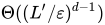
The latter result leaves a gap in the exponent. Chen and Deng closed the gap. They proved that, for any d ≥ 2 and $1/\varepsilon >4d$ and $L'/\varepsilon >192d^{3}$ , the number of queries required for computing an ε-residual fixed-point is in $\Theta ((L'/\varepsilon )^{d-1})$ .

05Discrete fixed-point computation

A discrete function is a function defined on a subset of $\mathbb {Z} ^{d}$ (the d-dimensional integer grid). There are several discrete fixed-point theorems, stating conditions under which a discrete function has a fixed point. For example, the Iimura-Murota-Tamura theorem states that (in particular) if $f$ is a function from a rectangle subset of $\mathbb {Z} ^{d}$ to itself, and $f$ is hypercubic direction-preserving, then $f$ has a fixed point.

Let $f$ be a direction-preserving function from the integer cube $\{1,\dots ,n\}^{d}$ to itself. Chen and Deng prove that, for any d ≥ 2 and n > 48d, computing such a fixed point requires $\Theta (n^{d-1})$ function evaluations.

Chen and Deng define a different discrete-fixed-point problem, which they call 2D-BROUWER. It considers a discrete function $f$ on $\{0,\dots ,n\}^{2}$ such that, for every x on the grid, $f$ (x) - x is either (0, 1) or (1, 0) or (-1, -1). The goal is to find a square in the grid, in which all three labels occur. The function $f$ must map the square $\{0,\dots ,n\}^{2}$ to itself, so it must map the lines x = 0 and y = 0 to either (0, 1) or (1, 0); the line x = n to either (-1, -1) or (0, 1); and the line y = n to either (-1, -1) or (1,0). The problem can be reduced to 2D-SPERNER (computing a fully-labeled triangle in a triangulation satisfying the conditions to Sperner's lemma), and therefore it is PPAD-complete. This implies that computing an approximate fixed-point is PPAD-complete even for very simple functions.

06Relation between fixed-point computation and root-finding algorithms

Given a function $g$ from $E^{d}$ to R, a root of $g$ is a point x in $E^{d}$ such that $g$ (x)=0. An ε-root of g is a point x in $E^{d}$ such that $g(x)\leq \varepsilon$ .

Fixed-point computation is a special case of root-finding: given a function $f$ on $E^{d}$ , define $g(x):=|f(x)-x|$ . X is a fixed-point of $f$ if and only if x is a root of $g$ , and x is an ε-residual fixed-point of $f$ if and only if x is an ε-root of $g$ . Therefore, any root-finding algorithm (an algorithm that computes an approximate root of a function) can be used to find an approximate fixed-point.

The opposite is not true: finding an approximate root of a general function may be harder than finding an approximate fixed point. In particular, Sikorski proved that finding an ε-root requires $\Omega (1/\varepsilon ^{d})$ function evaluations. This gives an exponential lower bound even for a one-dimensional function (in contrast, an ε-residual fixed-point of a one-dimensional function can be found using $O(\log(1/\varepsilon ))$ queries using the bisection method). Here is a proof sketch. Construct a function $g$ that is slightly larger than ε everywhere in $E^{d}$ except in some small cube around some point x₀, where x₀ is the unique root of $g$ . If $g$ is Lipschitz continuous with constant $L$ , then the cube around x₀ can have a side-length of $\varepsilon /L$ . Any algorithm that finds an ε-root of $g$ must check a set of cubes that covers the entire $E^{d}$ ; the number of such cubes is at least $(L/\varepsilon )^{d}$ .

However, there are classes of functions for which finding an approximate root is equivalent to finding an approximate fixed point. One example is the class of functions $g$ such that $g(x)+x$ maps $E^{d}$ to itself (that is: $g(x)+x$ is in $E^{d}$ for all x in $E^{d}$ ). This is because, for every such function, the function $f(x):=g(x)+x$ satisfies the conditions of Brouwer's fixed-point theorem. X is a fixed-point of $f$ if and only if x is a root of $g$ , and x is an ε-residual fixed-point of $f$ if and only if x is an ε-root of $g$ . Chen and Deng show that the discrete variants of these problems are computationally equivalent: both problems require $\Theta (n^{d-1})$ function evaluations.

07Communication complexity

Roughgarden and Weinstein studied the communication complexity of computing an approximate fixed-point. In their model, there are two agents: one of them knows a function $f$ and the other knows a function $g$ . Both functions are Lipschitz continuous and satisfy Brouwer's conditions. The goal is to compute an approximate fixed point of the composite function $g\circ f$ . They show that the deterministic communication complexity is in $\Omega (2^{d})$ .

Watch videos about Fixed-point computationExplainers and documentaries on YouTube (opens in a new tab)

Sources and credits

This article is adapted from the Wikipedia article “Fixed-point computation”, written by its contributors and licensed under CC BY-SA 4.0. Fathomly has changed the layout, removed citation markers, navigation and maintenance notices, and adjusted punctuation. This adapted version is shared under the same license. For references, see the original article.

Images, from Wikimedia Commons:

Fixed point example.svg by Krishnavedala, CC0
Fixed point anime.gif by Picknick, CC BY-SA 4.0

Fathomly is not affiliated with or endorsed by the Wikimedia Foundation. Spotted a problem? Tell us.