Sphere of influence (astrodynamics)
Region of space gravitationally dominated by a given body
A sphere of influence (SOI) in astrodynamics and astronomy is the oblate spheroid-shaped region where a particular celestial body exerts the main gravitational influence on an orbiting object. As such it is the dominating part of a gravitational field. It is usually used to describe the areas in the Solar System where planets dominate the orbits of surrounding objects such as moons, despite the presence of the much more massive but distant Sun.
In the patched conic approximation, used in estimating the trajectories of bodies moving between the neighbourhoods of different bodies using a two-body approximation, ellipses and hyperbolae, the SOI is taken as the boundary where the trajectory switches which mass field it is influenced by. It is not to be confused with the sphere of activity which extends well beyond the sphere of influence.
01Models
The most common base models to calculate the sphere of influence (sometimes also called gravisphere or gravity sphere) are the Hill sphere and the Laplace sphere, but updated and other models, as by Gleb Chebotaryov or particularly more dynamic ones, like the patched conic approximation, have been described. The general equation describing the radius of the sphere 
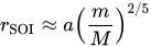
is the semimajor axis of the smaller object's (usually a planet's) orbit around the larger body (usually the Sun).
and
are the masses of the smaller and the larger object (usually a planet and the Sun), respectively.
In the patched conic approximation, once an object leaves the planet's SOI, the primary/only gravitational influence is the Sun (until the object enters another body's SOI). Because the definition of rSOI relies on the presence of the Sun and a planet, the term is only applicable in a three-body or greater system and requires the mass of the primary body to be much greater than the mass of the secondary body. This changes the three-body problem into a restricted two-body problem.

02Table of selected SOI radii
The table shows the values of the sphere of gravity of the bodies of the solar system in relation to the Sun (with the exception of the Moon which is reported relative to Earth):
| Body | SOI | Body Diameter | Body Mass (1024 kg) | Distance from Sun | |||||
|---|---|---|---|---|---|---|---|---|---|
| (106 km) | (mi) | (radii) | (km) | (mi) | (AU) | (106 mi) | (106 km) | ||
| Mercury | 0.117 | 72,700 | 46 | 4,878 | 3,031 | 0.33 | 0.39 | 36 | 57.9 |
| Venus | 0.616 | 382,765 | 102 | 12,104 | 7,521 | 4.867 | 0.723 | 67.2 | 108.2 |
| Earth + Moon | 0.929 | 577,254 | 145 | 12,742 (Earth) | 7,918 (Earth) | 5.972 (Earth) | 1 | 93 | 149.6 |
| Moon | 0.0643 | 39,993 | 37 | 3,476 | 2,160 | 0.07346 | See Earth + Moon | ||
| Mars | 0.578 | 359,153 | 170 | 6,780 | 4,212 | 0.65 | 1.524 | 141.6 | 227.9 |
| Jupiter | 48.2 | 29,950,092 | 687 | 139,822 | 86,881 | 1900 | 5.203 | 483.6 | 778.3 |
| Saturn | 54.5 | 38,864,730 | 1025 | 116,464 | 72,367 | 570 | 9.539 | 886.7 | 1,427.0 |
| Uranus | 51.9 | 32,249,165 | 2040 | 50,724 | 31,518 | 87 | 19.18 | 1,784.0 | 2,871.0 |
| Neptune | 86.2 | 53,562,197 | 3525 | 49,248 | 30,601 | 100 | 30.06 | 2,794.4 | 4,497.1 |
An important understanding to be drawn from this table is that "Sphere of Influence" here is "Primary". For example, though Jupiter is much larger in mass than Neptune, its Primary SOI is much smaller due to Jupiter's closer proximity to the Sun.

03Increased accuracy on the SOI
The sphere of influence is, in fact, not quite a sphere. The distance to the SOI depends on the angular distance 
![r_{\text{SOI}}(\theta )\approx a\left({\frac {m}{M}}\right)^{2/5}{\frac {1}{\sqrt[{10}]{1+3\cos ^{2}(\theta )}}}](https://wikimedia.org/api/rest_v1/media/math/render/svg/05a5c6c2fe78947b0074f5e9b7e2bffab910ec63)
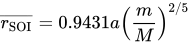
Averaging over all possible directions yields:

04Derivation
Consider two point masses 


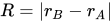


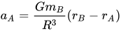
Consider a frame centered on 

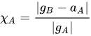


| Frame A | Frame B | |
|---|---|---|
| Main acceleration | | |
| Frame acceleration |  |  |
| Secondary acceleration | | |
| Perturbation, tidal forces | |  |
Perturbation ratio  | | 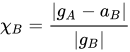 |
As 


| Frame A | Frame B | |
|---|---|---|
| Main acceleration |  |  |
| Frame acceleration |  | 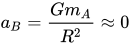 |
| Secondary acceleration | 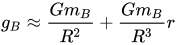 | |
| Perturbation, tidal forces | 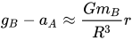 | 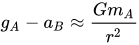 |
| Perturbation ratio | 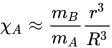 | 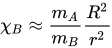 |
The distance to the sphere of influence must thus satisfy 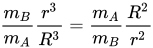
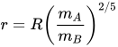

05Gravity well
A gravity well (or funnel) is a metaphorical concept for a gravitational field of a mass, with the field being curved in a funnel-shaped well around the mass, illustrating the steep gravitational potential and its energy that needs to be accounted for in order to escape or enter the main part of a sphere of influence.
An example for this is the strong gravitational field of the Sun and Mercury being deep within it. At perihelion Mercury goes even deeper into the Sun's gravity well, causing an anomalistic or perihelion apsidal precession which is more recognizable than with other planets due to Mercury being deep in the gravity well. This characteristic of Mercury's orbit was famously calculated by Albert Einstein through his formulation of gravity with the speed of light, and the corresponding general relativity theory, eventually being one of the first cases proving the theory.

06General references
- Bate, Roger R.; Mueller, Donald D.; White, Jerry E. (1971). Fundamentals of astrodynamics. Dover books on astronomy. New York: Dover Publications. pp. 333-334. ISBN 978-0-486-60061-1.
- Sellers, Jerry Jon; Astore, William J.; Giffen, Robert B.; Larson, Wiley J. (2015). Marilyn (ed.). Understanding space: an introduction to astronautics (4nd ed.). New York: McGraw-Hill Companies. pp. 228, 738. ISBN 978-0-9904299-4-4.
- Danby, J. M. A. (1992). Fundamentals of celestial mechanics (2nd ed.). Richmond, Va., U.S.A: Willmann-Bell. pp. 352, 353. ISBN 978-0-943396-20-0.
Sources and credits
This article is adapted from the Wikipedia article “Sphere of influence (astrodynamics)”, written by its contributors and licensed under CC BY-SA 4.0. Fathomly has changed the layout, removed citation markers, navigation and maintenance notices, and adjusted punctuation. This adapted version is shared under the same license. For references, see the original article.
Images, from Wikimedia Commons:
- Sphere of influence on ratio m M.png by Lamid58, CC BY-SA 4.0
- Sphereofinfluence.png by Agnity, CC BY-SA 4.0
- Hill sphere and SOI.png by Lamid58, CC BY-SA 4.0
- Gravitational Well.gif by NectarLupine, CC0
- Schwarzschild effective potential.svg by No machine-readable author provided. Cronholm144 assumed (based on copyright claims)., CC BY-SA 3.0
Fathomly is not affiliated with or endorsed by the Wikimedia Foundation. Spotted a problem? Tell us.
