Encyclopedia

Generalised logistic function

Mathematical function

Wikipedia contributorsAdapted for Fathomly · View authors

1 min read
Source updated February 23, 2026

Image credit is listed at the end of this article.

The generalized logistic function or curve is an extension of the logistic or sigmoid functions. Originally developed for growth modelling, it allows for more flexible S-shaped curves. The function is sometimes named Richards's curve after F. J. Richards, who proposed the general form for the family of models in 1959.

01Definition

Richards's curve has the following form:

$Y(t)=A+{K-A \over (C+Qe^{-Bt})^{1/\nu }}$

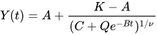
where $Y$ = weight, height, size etc., and $t$ = time. It has six parameters:

$A$ : the left horizontal asymptote;
$K$ : the right horizontal asymptote when $C=1$ . If $A=0$ and $C=1$ then $K$ is called the carrying capacity;
$B$ : the growth rate;
$\nu >0$ : affects near which asymptote maximum growth occurs.
$Q$ : is related to the value $Y(0)$
$C$ : typically takes a value of 1. Otherwise, the upper asymptote is $A+{K-A \over C^{\,1/\nu }}$

The equation can also be written:

$Y(t)=A+{K-A \over (C+e^{-B(t-M)})^{1/\nu }}$

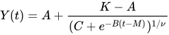
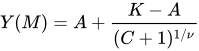
where $M$ can be thought of as a starting time, at which $Y(M)=A+{K-A \over (C+1)^{1/\nu }}$ . Including both $Q$ and $M$ can be convenient:

$Y(t)=A+{K-A \over (C+Qe^{-B(t-M)})^{1/\nu }}$

this representation simplifies the setting of both a starting time and the value of $Y$ at that time.

The logistic function, with maximum growth rate at time $M$ , is the case where $Q=\nu =1$ .

Effect of varying parameter A. All other parameters are 1.

Effect of varying parameter B. A = 0, all other parameters are 1.

02Generalised logistic differential equation

A particular case of the generalised logistic function is:

$Y(t)={K \over (1+Qe^{-\alpha \nu (t-t_{0})})^{1/\nu }}$

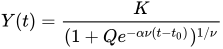
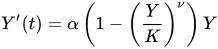
which is the solution of the Richards's differential equation (RDE):

$Y^{\prime }(t)=\alpha \left(1-\left({\frac {Y}{K}}\right)^{\nu }\right)Y$

with initial condition

$Y(t_{0})=Y_{0}$

where

$Q=-1+\left({\frac {K}{Y_{0}}}\right)^{\nu }$

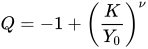
provided that $\nu >0$ and $\alpha >0$

The classical logistic differential equation is a particular case of the above equation, with $\nu =1$ , whereas the Gompertz curve can be recovered in the limit $\nu \rightarrow 0^{+}$ provided that:

$\alpha =O\left({\frac {1}{\nu }}\right)$

In fact, for small $\nu$ it is

$Y^{\prime }(t)=Yr{\frac {1-\exp \left(\nu \ln \left({\frac {Y}{K}}\right)\right)}{\nu }}\approx rY\ln \left({\frac {Y}{K}}\right)$

The RDE models many growth phenomena, arising in fields such as oncology and epidemiology.

Effect of varying parameter C. A = 0, all other parameters are 1.

03Gradient of generalized logistic function

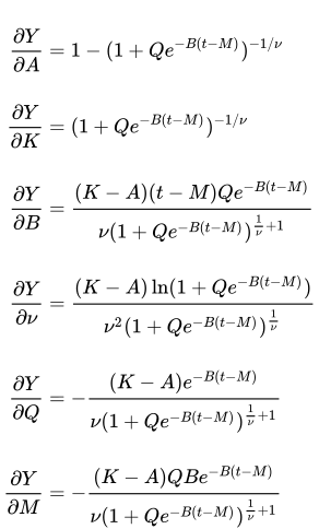
When estimating parameters from data, it is often necessary to compute the partial derivatives of the logistic function with respect to parameters at a given data point $t$ (see). For the case where $C=1$ ,

${\begin{aligned}\\{\frac {\partial Y}{\partial A}}&=1-(1+Qe^{-B(t-M)})^{-1/\nu }\\\\{\frac {\partial Y}{\partial K}}&=(1+Qe^{-B(t-M)})^{-1/\nu }\\\\{\frac {\partial Y}{\partial B}}&={\frac {(K-A)(t-M)Qe^{-B(t-M)}}{\nu (1+Qe^{-B(t-M)})^{{\frac {1}{\nu }}+1}}}\\\\{\frac {\partial Y}{\partial \nu }}&={\frac {(K-A)\ln(1+Qe^{-B(t-M)})}{\nu ^{2}(1+Qe^{-B(t-M)})^{\frac {1}{\nu }}}}\\\\{\frac {\partial Y}{\partial Q}}&=-{\frac {(K-A)e^{-B(t-M)}}{\nu (1+Qe^{-B(t-M)})^{{\frac {1}{\nu }}+1}}}\\\\{\frac {\partial Y}{\partial M}}&=-{\frac {(K-A)QBe^{-B(t-M)}}{\nu (1+Qe^{-B(t-M)})^{{\frac {1}{\nu }}+1}}}\\\end{aligned}}$

Effect of varying parameter K. A = 0, all other parameters are 1.

Effect of varying parameter Q. A = 0, all other parameters are 1.

04Special cases

The following functions are specific cases of Richards's curves:

Effect of varying parameter . A = 0, all other parameters are 1.

Watch videos about Generalised logistic functionExplainers and documentaries on YouTube (opens in a new tab)

Sources and credits

This article is adapted from the Wikipedia article “Generalised logistic function”, written by its contributors and licensed under CC BY-SA 4.0. Fathomly has changed the layout, removed citation markers, navigation and maintenance notices, and adjusted punctuation. This adapted version is shared under the same license. For references, see the original article.

Images, from Wikimedia Commons:

Generalized logistic function A0 K1 B1.5 Q0.5 ν0.5 M0.5.png by Debiatan at en.wikipedia, Public domain
GeneralizedLogisticA.svg by Bbanerje at English Wikipedia, CC BY-SA 3.0
GeneralizedLogisticB.svg by Bbanerje at English Wikipedia, CC BY-SA 3.0
GeneralizedLogisticC.svg by Bbanerje at English Wikipedia, CC BY-SA 3.0
GeneralizedLogisticK.svg by Bbanerje at English Wikipedia, CC BY-SA 3.0
GeneralizedLogisticQ.svg by Bbanerje at English Wikipedia, CC BY-SA 3.0
GeneralizedLogisticNu.svg by Bbanerje at English Wikipedia, CC BY-SA 3.0

Fathomly is not affiliated with or endorsed by the Wikimedia Foundation. Spotted a problem? Tell us.