Encyclopedia

Generalized functional linear model

Mathematical model for stochastic processes

Wikipedia contributorsAdapted for Fathomly · View authors

7 min read
Source updated September 27, 2025

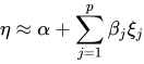
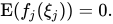
The generalized functional linear model (GFLM) is an extension of the generalized linear model (GLM) that allows one to regress univariate responses of various types (continuous or discrete) on functional predictors, which are mostly random trajectories generated by a square-integrable stochastic processes. Similarly to GLM, a link function relates the expected value of the response variable to a linear predictor, which in case of GFLM is obtained by forming the scalar product of the random predictor function $X$ with a smooth parameter function $\beta$ . Functional Linear Regression, Functional Poisson Regression and Functional Binomial Regression, with the important Functional Logistic Regression included, are special cases of GFLM. Applications of GFLM include classification and discrimination of stochastic processes and functional data.

01Overview

A key aspect of GFLM is estimation and inference for the smooth parameter function $\beta$ which is usually obtained by dimension reduction of the infinite dimensional functional predictor. A common method is to expand the predictor function $X$ in an orthonormal basis of L² space, the Hilbert space of square integrable functions with the simultaneous expansion of the parameter function in the same basis. 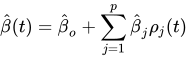This representation is then combined with a truncation step to reduce the contribution of the parameter function $\beta$ in the linear predictor to a finite number of regression coefficients. Functional principal component analysis (FPCA) that employs the Karhunen-Loève expansion is a common and parsimonious approach to accomplish this. Other orthogonal expansions, like Fourier expansions and B-spline expansions may also be employed for the dimension reduction step. The Akaike information criterion (AIC) can be used for selecting the number of included components. Minimization of cross-validation prediction errors is another criterion often used in classification applications. Once the dimension of the predictor process has been reduced, the simplified linear predictor allows to use GLM and quasi-likelihood estimation techniques to obtain estimates of the finite dimensional regression coefficients which in turn provide an estimate of the parameter function $\beta$ in the GFLM.

02Model components

Linear predictor

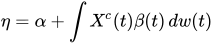
The predictor functions $\textstyle X(t),t\in T$ , typically are square integrable stochastic processes on a real interval $T$ and the unknown smooth parameter function $\beta (t),t\in T$ , is assumed to be square integrable on $T$ . Given a real measure $dw$ on $T$ , the linear predictor is given by $\eta =\alpha +\int X^{c}(t)\beta (t)\,dw(t)$ where $X^{c}(t)=X(t)-{\text{E}}(X(t))$ is the centered predictor process and $\alpha$ is a scalar that serves as an intercept.

Response variable and variance function

The outcome $Y$ is typically a real valued random variable which may be either continuous or discrete. Often the conditional distribution of $Y$ given the predictor process is specified within the exponential family. 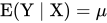However it is also sufficient to consider the functional quasi-likelihood set up, where instead of the distribution of the response one specifies the conditional variance function, ${\rm {{Var}(Y\mid X)=\sigma ^{2}(\mu )}}$ , as a function of the conditional mean, ${\rm {{E}(Y\mid X)=\mu }}$ .

Link function

The link function $g$ is a smooth invertible function, that relates the conditional mean of the response ${\rm {{E}(Y\mid X)=\mu }}$ with the linear predictor $\eta =\alpha +\int X^{c}(t)\beta (t)\,dw(t)$ . The relationship is given by $\mu =g(\eta )$ .

03Formulation

In order to implement the necessary dimension reduction, the centered predictor process $X^{c}(t)$ and the parameter function $\beta (t)$ are expanded as,

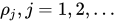
$X^{c}(t)=\sum _{j=1}^{\infty }\xi _{j}\rho _{j}(t){\text{ and }}\beta (t)=\sum _{j=1}^{\infty }\beta _{j}\rho _{j}(t),$

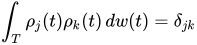
where $\rho _{j},j=1,2,\ldots$ is an orthonormal basis of the function space $L^{2}(dw),$ such that $\int _{T}\rho _{j}(t)\rho _{k}(t)\,dw(t)=\delta _{jk}$ where $\delta _{jk}=1$ if $j=k$ and $0$ otherwise.

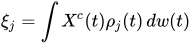
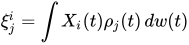
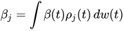
The random variables $\xi _{j}$ are given by $\xi _{j}=\int X^{c}(t)\rho _{j}(t)\,dw(t)$ and the coefficients $\beta _{j}$ as $\beta _{j}=\int \beta (t)\rho _{j}(t)\,dw(t)$ for $j=1,2,\ldots$ .

${\text{E}}(\xi _{j})=0$ and $\sum _{j=1}^{\infty }\beta _{j}^{2}<\infty$ and denoting $\sigma _{j}^{2}={\text{Var}}(\xi _{j})={\text{E}}(\xi _{j}^{2})$ , so $\sum _{j=1}^{\infty }\sigma _{j}^{2}=\int {\text{E}}(X^{c}(t))^{2}\,dw(t)<\infty$ .

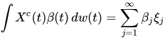
From the orthonormality of the basis functions $\rho _{j}$ , it follows immediately that $\int X^{c}(t)\beta (t)\,dw(t)=\sum _{j=1}^{\infty }\beta _{j}\xi _{j}$ .

The key step is then approximating $\eta =\alpha +\int X^{c}(t)\beta (t)\,dw(t)=\alpha +\sum _{j=1}^{\infty }\beta _{j}\xi _{j}$ by $\eta \approx \alpha +\sum _{j=1}^{p}\beta _{j}\xi _{j}$ for a suitably chosen truncation point $p$ .

FPCA gives the most parsimonious approximation of the linear predictor for a given number of basis functions as the eigenfunction basis explains more of the variation than any other set of basis functions.

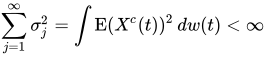
For a differentiable link function with bounded first derivative, the approximation error of the $p$ -truncated model i.e. the linear predictor truncated to the summation of the first $p$ components, is a constant multiple of ${\text{Var}}(\sum _{j=p+1}^{\infty }\beta _{j}\xi _{j})={\text{E}}\left(\left(\sum _{j=p+1}^{\infty }\beta _{j}\xi _{j}\right)^{2}\right)=\sum _{j=p+1}^{\infty }\beta _{j}\sigma _{j}^{2}$ .

A heuristic motivation for the truncation strategy derives from the fact that ${\text{E}}\left(\left(\sum _{j=p+1}^{\infty }\beta _{j}\xi _{j}\right)^{2}\right)=\sum _{j=p+1}^{\infty }\beta _{j}\sigma _{j}^{2}\leq \sum _{j=p+1}^{\infty }\beta _{j}^{2}\ \sum _{j=p+1}^{\infty }\sigma _{j}^{2}$ which is a consequence of the Cauchy-Schwarz inequality and by noting that the right hand side of the last inequality converges to 0 as $p\rightarrow \infty$ since both $\sum _{j=1}^{\infty }\beta _{j}^{2}$ and $\sum _{j=1}^{\infty }\sigma _{j}^{2}$ are finite.

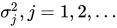
For the special case of the eigenfunction basis, the sequence $\sigma _{j}^{2},j=1,2,\ldots$ corresponds to the sequence of the eigenvalues of the covariance kernel $G(s,t)={\text{Cov}}(X(s),X(t)),\ s,t\in T$ .

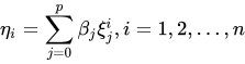
For data with $n$ i.i.d observations, setting $\xi _{j}^{0}=1$ , $\beta _{0}=\alpha$ and $\xi _{j}^{i}=\int X_{i}(t)\rho _{j}(t)\,dw(t)$ , the approximated linear predictors can be represented as $\eta _{i}=\sum _{j=0}^{p}\beta _{j}\xi _{j}^{i},i=1,2,\ldots ,n$ which are related to the means through $\mu _{i}=g(\eta _{i})$ .

04Estimation

The main aim is to estimate the parameter function $\beta$ .

Once $p$ has been fixed, standard GLM and quasi-likelihood methods can be used for the $p$ -truncated model to estimate ${\boldsymbol {\beta }}^{T}=(\beta _{0},\beta _{1},\ldots ,\beta _{p})$ by solving the estimating equation or the score equation $U(\beta )=0.$

The vector valued score function turns out to be $U(\beta )=\sum _{i=1}^{n}(Y_{i}-\mu _{i})g'(\eta _{i})\xi _{i}/\sigma ^{2}(\mu _{i})$ which depends on ${\boldsymbol {\beta }}$ through $\mu$ and $\eta$ .

Just as in GLM, the equation $U(\beta )=0$ is solved using iterative methods like Newton-Raphson (NR) or Fisher scoring (FS) or iteratively reweighted least squares (IWLS) to get the estimate of the regression coefficients ${\boldsymbol {\hat {\beta }}}$ , leading to the estimate of the parameter function ${\hat {\beta }}(t)={\hat {\beta }}_{o}+\sum _{j=1}^{p}{\hat {\beta }}_{j}\rho _{j}(t)$ . When using the canonical link function, these methods are equivalent.

Results are available in the literature of $p$ -truncated models as $p\rightarrow \infty$ which provide asymptotic inference for the deviation of the estimated parametric function from the true parametric function and also asymptotic tests for regression effects and asymptotic confidence regions.

05Exponential family response

If the response variable $Y_{i}$ , given $X_{i}\in L^{2}(T)$ follows the one parameter exponential family, then its probability density function or probability mass function (as the case may be) is

$f(y_{i}\mid X_{i})=\exp \left({\frac {y_{i}\theta _{i}-b(\theta _{i})}{\phi }}+c(y_{i},\phi )\right)$

for some functions $b$ and $c$ , where $\theta _{i}$ is the canonical parameter, and $\phi$ is a dispersion parameter which is typically assumed to be positive.

In the canonical set up, $\eta _{i}=\alpha +\int X_{i}^{c}(t)\beta (t)\,dw(t)=\theta _{i}$ and from the properties of exponential family,

$\mu _{i}=b'(\theta _{i}),{\text{ and so }}\mu _{i}=b'(\eta _{i}).$

Hence $b'$ serves as a link function and is called the canonical link function.

${\text{Var}}(y_{i})=\phi b''(\theta _{i})=\phi b''(\eta _{i})=\phi g'(\eta _{i})=\phi g'(g^{-1}(\mu _{i})))$ is the corresponding variance function and $\phi$ the dispersion parameter.

06Special cases

Functional linear regression (FLR)

Functional linear regression, one of the most useful tools of functional data analysis, is an example of GFLM where the response variable is continuous and is often assumed to have a Normal distribution. The variance function is a constant function and the link function is identity. Under these assumptions the GFLM reduces to the FLR,

$\mu =\operatorname {E} (Y\mid X)=\eta =\alpha +\int X^{c}(t)\beta (t)\,dw(t)$

Without the normality assumption, the constant variance function motivates the use of quasi-normal techniques.

Functional binary regression

When the response variable has binary outcomes, i.e., 0 or 1, the distribution is usually chosen as Bernoulli, and then $\mu _{i}=P(Y_{i}=1\mid X_{i})$ . Popular link functions are the expit function, which is the inverse of the logit function (functional logistic regression) and the probit function (functional probit regression). Any cumulative distribution function F has range [0,1] which is the range of binomial mean and so can be chosen as a link function. Another link function in this context is the complementary log-log function, which is an asymmetric link. The variance function for binary data is given by $\operatorname {Var} (Y_{i})=\phi \mu _{i}(1-\mu _{i})$ where the dispersion parameter $\phi$ is taken as 1 or alternatively the quasi-likelihood approach is used.

Functional Poisson regression

Another special case of GFLM occurs when the outcomes are counts, so that the distribution of the responses is assumed to be Poisson. The mean $\mu _{i}$ is typically linked to the linear predictor $\eta _{i}$ via a log-link, which is also the canonical link . The variance function is $\operatorname {Var} (Y_{i})=\phi \mu _{i}$ , where the dispersion parameter $\phi$ is 1, except when the data might be over-dispersed which is when the quasi-Poisson approach is used.

07Extensions

Extensions of GFLM have been proposed for the cases where there are multiple predictor functions. Another generalization is called the Semi Parametric Quasi-likelihood Regression (SPQR) which considers the situation where the link and the variance functions are unknown and are estimated non-parametrically from the data. This situation can also be handled by single or multiple index models, using for example Sliced Inverse Regression (SIR).

Another extension in this domain is Functional Generalized Additive Model (FGAM)) which is a generalization of generalized additive model(GAM) where

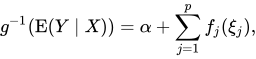
$g^{-1}(\operatorname {E} (Y\mid X))=\alpha +\sum _{j=1}^{p}f_{j}(\xi _{j}),$

where $\xi _{j}$ are the expansion coefficients of the random predictor function $X$ and each $f_{j}$ is an unknown smooth function that has to be estimated and where ${\text{E}}(f_{j}(\xi _{j}))=0.$ .

In general, estimation in FGAM requires combining IWLS with backfitting. However, if the expansion coefficients are obtained as functional principal components, then in some cases (e.g. Gaussian predictor function $X$ ), they will be independent in which case backfitting is not needed, and one can use popular smoothing methods for estimating the unknown parameter functions $f_{j}$ .

08Application

A popular data set that has been used for a number of analysis in the domain of functional data analysis consists of the number of eggs laid daily until death of 1000 Mediterranean fruit flies (or medflies for short) . The plot here shows the egg laying trajectories in the first 25 days of life of about 600 female medflies (those that have at least 20 remaining eggs in their lifetime). The red colored curves belong to those flies that will lay less than the median number of remaining eggs, while the blue colored curves belong to the flies that will lay more than the median number of remaining eggs after age 25. A related problem of classifying medflies as long-lived or short-lived based on the initial egg laying trajectories as predictors and the subsequent longevity of the flies as response has been studied with the GFLM

Watch videos about Generalized functional linear modelExplainers and documentaries on YouTube (opens in a new tab)

Sources and credits

This article is adapted from the Wikipedia article “Generalized functional linear model”, written by its contributors and licensed under CC BY-SA 4.0. Fathomly has changed the layout, removed citation markers, navigation and maintenance notices, and adjusted punctuation. This adapted version is shared under the same license. For references, see the original article.

Images, from Wikimedia Commons:

Egg Laying Trajectories of Medflies.png by Dragon warrior rises, CC BY-SA 4.0

Fathomly is not affiliated with or endorsed by the Wikimedia Foundation. Spotted a problem? Tell us.