Fresnel integral
Special function defined by an integral

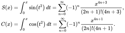
The Fresnel integrals S(x) and C(x), and their auxiliary functions F(x) and G(x) are transcendental functions named after Augustin-Jean Fresnel that are used in optics and are closely related to the error function (erf). They arise in the description of near-field Fresnel diffraction phenomena and are defined through the following integral representations:

The parametric curve 
The term Fresnel integral may also refer to the complex definite integral

where a is real and positive; this can be evaluated by closing a contour in the complex plane and applying Cauchy's integral theorem.
01Definition
The Fresnel integrals admit the following Maclaurin series that converge for all x:
Some widely used tables use π/2t2 instead of t2 for the argument of the integrals defining S(x) and C(x). This changes their limits at infinity from 1/2·√π/2 to 1/2 and the arc length for the first spiral turn from √2π to 2 (at t = 2). These alternative functions are usually known as normalized Fresnel integrals.
The Auxiliary functions F(x) and G(x) provide monotonic bounds for the Fresnel Integrals:

![Fresnel integrals with arguments 2</sup>"}},"i":0}}]}' id="mwMg">π/2t2 instead of 2</sup>"}},"i":0}}]}' id="mwMw">t2 converge to 1/2 instead of 1/2·√π⁄2.](https://thumb.wikimedia.org/wikipedia/commons/thumb/8/8f/Fresnel_Integrals_%28Normalised%29.svg/500px-Fresnel_Integrals_%28Normalised%29.svg.png)
02Euler spiral
The Euler spiral, also known as a Cornu spiral or clothoid, is the curve generated by a parametric plot of S(t) against C(t). The Euler spiral was first studied in the mid 18th century by Leonhard Euler in the context of Euler-Bernoulli beam theory. A century later, Marie Alfred Cornu constructed the same spiral as a nomogram for diffraction computations.
From the definitions of Fresnel integrals, the infinitesimals dx and dy are thus:
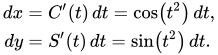
Thus the length of the spiral measured from the origin can be expressed as

That is, the parameter t is the curve length measured from the origin (0, 0), and the Euler spiral has infinite length. The vector (cos(t2), sin(t2)), where θ = t2, also expresses the unit tangent vector along the spiral. Since t is the curve length, the curvature κ can be expressed as
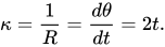
Thus the rate of change of curvature with respect to the curve length is

An Euler spiral has the property that its curvature at any point is proportional to the distance along the spiral, measured from the origin. This property makes it useful as a transition curve in highway and railway engineering: if a vehicle follows the spiral at unit speed, the parameter t in the above derivatives also represents the time. Consequently, a vehicle following the spiral at constant speed will have a constant rate of angular acceleration.
Sections from Euler spirals are commonly incorporated into the shape of rollercoaster loops to make what are known as clothoid loops.

03Properties
C(x) and S(x) are odd functions of x,

which can be readily seen from the fact that their power series expansions have only odd-degree terms, or alternatively because they are antiderivatives of even functions that also are zero at the origin.
Asymptotics of the Fresnel integrals as x → ∞ are given by the formulas:
![{\begin{aligned}S(x)&={\sqrt {{\tfrac {1}{8}}\pi }}\operatorname {sgn} x-\left[1+O\left(x^{-4}\right)\right]\left({\frac {\cos \left(x^{2}\right)}{2x}}+{\frac {\sin \left(x^{2}\right)}{4x^{3}}}\right),\\[6px]C(x)&={\sqrt {{\tfrac {1}{8}}\pi }}\operatorname {sgn} x+\left[1+O\left(x^{-4}\right)\right]\left({\frac {\sin \left(x^{2}\right)}{2x}}-{\frac {\cos \left(x^{2}\right)}{4x^{3}}}\right).\end{aligned}}](https://wikimedia.org/api/rest_v1/media/math/render/svg/971e463cafda1adb8f69182c12bb2a812495215e)
Using the power series expansions above, the Fresnel integrals can be extended to the domain of complex numbers, where they become entire functions of the complex variable z.
The Fresnel integrals can be expressed using the error function as follows:
![{\begin{aligned}S(z)&={\sqrt {\frac {\pi }{2}}}\cdot {\frac {1+i}{4}}\left[\operatorname {erf} \left({\frac {1+i}{\sqrt {2}}}z\right)-i\operatorname {erf} \left({\frac {1-i}{\sqrt {2}}}z\right)\right],\\[6px]C(z)&={\sqrt {\frac {\pi }{2}}}\cdot {\frac {1-i}{4}}\left[\operatorname {erf} \left({\frac {1+i}{\sqrt {2}}}z\right)+i\operatorname {erf} \left({\frac {1-i}{\sqrt {2}}}z\right)\right].\end{aligned}}](https://wikimedia.org/api/rest_v1/media/math/render/svg/407600705c2052e6eb7040fa8557b62d68057988)
or
![{\begin{aligned}C(z)+iS(z)&={\sqrt {\frac {\pi }{2}}}\cdot {\frac {1+i}{2}}\operatorname {erf} \left({\frac {1-i}{\sqrt {2}}}z\right),\\[6px]S(z)+iC(z)&={\sqrt {\frac {\pi }{2}}}\cdot {\frac {1+i}{2}}\operatorname {erf} \left({\frac {1+i}{\sqrt {2}}}z\right).\end{aligned}}](https://wikimedia.org/api/rest_v1/media/math/render/svg/2d8ce089075b919154f476c7ce03d0042de5d9d0)
Limits as x approaches infinity
The integrals defining C(x) and S(x) cannot be evaluated in the closed form in terms of elementary functions, except in special cases. The limits of these functions as x goes to infinity are known:

| Proof of the formula |
|---|
|
This can be derived with any one of several methods. One of them uses a contour integral of the function As R goes to infinity, the integral along the circular arc γ2 tends to 0
Note too that because the integrand is an entire function on the complex plane, its integral along the whole contour is zero by the Cauchy integral theorem. Overall, we must have
Using Euler's formula to take real and imaginary parts of e−it2 gives this as
Solving this for IC and IS gives the desired result. |
 around the boundary of the
  where polar coordinates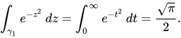
 where
where 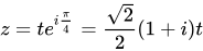 where
where 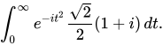
![{\begin{aligned}&\int _{0}^{\infty }\left(\cos \left(t^{2}\right)-i\sin \left(t^{2}\right)\right){\frac {\sqrt {2}}{2}}(1+i)\,dt\\[6px]&\quad ={\frac {\sqrt {2}}{2}}\int _{0}^{\infty }\left[\cos \left(t^{2}\right)+\sin \left(t^{2}\right)+i\left(\cos \left(t^{2}\right)-\sin \left(t^{2}\right)\right)\right]\,dt\\[6px]&\quad ={\frac {\sqrt {\pi }}{2}}+0i,\end{aligned}}](https://wikimedia.org/api/rest_v1/media/math/render/svg/d989e74dd984a8127b5f034eb8392d61d3101790) where we have written
where we have written  and then equating real and imaginary parts produces the following system of two equations in the two unknowns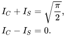

04Generalization
The integral

![{\begin{aligned}\int x^{m}e^{ix^{n}}\,dx&={\frac {x^{m+1}}{m+1}}\,_{1}F_{1}\left({\begin{array}{c}{\frac {m+1}{n}}\\1+{\frac {m+1}{n}}\end{array}}\mid ix^{n}\right)\\[6px]&={\frac {1}{n}}i^{\frac {m+1}{n}}\gamma \left({\frac {m+1}{n}},-ix^{n}\right),\end{aligned}}](https://wikimedia.org/api/rest_v1/media/math/render/svg/2e48d28903c53cdfc707c5b0c92a08bdc4612b0c)



For m = 0, the imaginary part of this equation in particular is

The Kummer transformation of the confluent hypergeometric function is
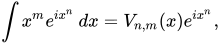


05Numerical approximation
For computation to arbitrary precision, the power series is suitable for small argument. For large argument, asymptotic expansions converge faster. Continued fraction methods may also be used.
For computation to particular target precision, other approximations have been developed. William J. Cody developed a set of efficient approximations based on rational functions that give relative errors down to 2×10⁻¹⁹. A FORTRAN implementation of the Cody approximation that includes the values of the coefficients needed for implementation in other languages was published by van Snyder. Boersma developed an approximation with error less than 1.6×10⁻⁹.

06Applications
The Fresnel integrals were originally used in the calculation of the electromagnetic field intensity in an environment where light bends around opaque objects. More recently, they have been used in the design of highways and railways, specifically their curvature transition zones, see track transition curve. Other applications are rollercoasters or calculating the transitions on a velodrome track to allow rapid entry to the bends and gradual exit.

Sources and credits
This article is adapted from the Wikipedia article “Fresnel integral”, written by its contributors and licensed under CC BY-SA 4.0. Fathomly has changed the layout, removed citation markers, navigation and maintenance notices, and adjusted punctuation. This adapted version is shared under the same license. For references, see the original article.
Images, from Wikimedia Commons:
- Fresnel Integrals (Unnormalised).svg by Inductiveload, Public domain
- Fresnel Integrals (Normalised).svg by Inductiveload, Public domain
- Cornu Spiral.svg by Inductiveload, Public domain
- CornuSpiralAnimation.gif by Mkwadee, CC BY-SA 3.0
- Fresnel S with domain coloring.svg by Nschloe, CC BY-SA 4.0
- Fresnel C with domain coloring.svg by Nschloe, CC BY-SA 4.0
- Fresnel Integral Contour.svg by Inductiveload, Public domain
Fathomly is not affiliated with or endorsed by the Wikimedia Foundation. Spotted a problem? Tell us.

