Encyclopedia

Feigenbaum function

Concept in dynamical systems

Wikipedia contributorsAdapted for Fathomly · View authors

3 min read
Source updated September 7, 2026

In the study of dynamical systems the term Feigenbaum function has been used to describe two different functions introduced by the physicist Mitchell Feigenbaum:

the solution to the Feigenbaum-Cvitanović functional equation; and
the scaling function that described the covers of the attractor of the logistic map

01Idea

Period-doubling route to chaos

In the logistic map,

$x_{n+1}=rx_{n}(1-x_{n}),$

we have a function $f_{r}(x)=rx(1-x)$ , and we want to study what happens when we iterate the map many times. The map might fall into a fixed point, a fixed cycle, or chaos. When the map falls into a stable fixed cycle of length $n$ , we would find that the graph of $f_{r}^{n}$ and the graph of $x\mapsto x$ intersects at $n$ points, and the slope of the graph of $f_{r}^{n}$ is bounded in $(-1,+1)$ at those intersections.

For example, when $r=3.0$ , we have a single intersection, with slope bounded in $(-1,+1)$ , indicating that it is a stable single fixed point.

As $r$ increases to beyond $r=3.0$ , the intersection point splits to two, which is a period doubling. For example, when $r=3.4$ , there are three intersection points, with the middle one unstable, and the two others stable.

As $r$ approaches $r=3.45$ , another period-doubling occurs in the same way. The period-doublings occur more and more frequently, until at a certain $r\approx 3.56994567$ , the period doublings become infinite, and the map becomes chaotic. This is the period-doubling route to chaos.

Scaling limit

Looking at the images, one can notice that at the point of chaos $r^{*}=3.5699\cdots$ , the curve of $f_{r^{*}}^{\infty }$ looks like a fractal. Furthermore, as we repeat the period-doublings $f_{r^{*}}^{1},f_{r^{*}}^{2},f_{r^{*}}^{4},f_{r^{*}}^{8},f_{r^{*}}^{16},\dots$ , the graphs seem to resemble each other, except that they are shrunken towards the middle, and rotated by 180 degrees.

This suggests to us a scaling limit: if we repeatedly double the function, then scale it up by $\alpha$ for a certain constant $\alpha$ : $f(x)\mapsto -\alpha f(f(-x/\alpha ))$ then at the limit, we would end up with a function $g$ that satisfies $g(x)=-\alpha g(g(-x/\alpha ))$ . Further, as the period-doubling intervals become shorter and shorter, the ratio between two period-doubling intervals converges to a limit, the first Feigenbaum constant $\delta =4.6692016\cdots$ .

The constant $\alpha$ can be numerically found by trying many possible values. For the wrong values, the map does not converge to a limit, but when it is $\alpha =2.5029\dots$ , it converges. This is the second Feigenbaum constant.

Chaotic regime

In the chaotic regime, $f_{r}^{\infty }$ , the limit of the iterates of the map, becomes chaotic dark bands interspersed with non-chaotic bright bands.

Other scaling limits

When $r$ approaches $r\approx 3.8494344$ , we have another period-doubling approach to chaos, but this time with periods 3, 6, 12, ... This again has the same Feigenbaum constants $\delta ,\alpha$ . The limit of ${\textstyle f(x)\mapsto -\alpha f(f(-x/\alpha ))$ is also the same function. This is an example of universality.

We can also consider period-tripling route to chaos by picking a sequence of $r_{1},r_{2},\dots$ such that $r_{n}$ is the lowest value in the period- $3^{n}$ window of the bifurcation diagram. For example, we have $r_{1}=3.8284,r_{2}=3.85361,\dots$ , with the limit $r_{\infty }=3.854077963\dots$ . This has a different pair of Feigenbaum constants $\delta =55.26\dots ,\alpha =9.277\dots$ . And $f_{r}^{\infty }$ converges to the fixed point to $f(x)\mapsto -\alpha f(f(f(-x/\alpha )))$ As another example, period-4-pling has a pair of Feigenbaum constants distinct from that of period-doubling, even though period-4-pling is reached by two period-doublings. In detail, define $r_{1},r_{2},\dots$ such that $r_{n}$ is the lowest value in the period- $4^{n}$ window of the bifurcation diagram. Then we have $r_{1}=3.960102,r_{2}=3.9615554,\dots$ , with the limit $r_{\infty }=3.96155658717\dots$ . This has a different pair of Feigenbaum constants $\delta =981.6\dots ,\alpha =38.82\dots$ .

In general, each period-multiplying route to chaos has its own pair of Feigenbaum constants. In fact, there are typically more than one. For example, for period-7-pling, there are at least 9 different pairs of Feigenbaum constants.

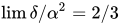
Generally, ${\textstyle 3\delta \approx 2\alpha ^{2}$ , and the relation becomes exact as both numbers increase to infinity: $\lim \delta /\alpha ^{2}=2/3$ .

02Feigenbaum-Cvitanović functional equation

This functional equation arises in the study of one-dimensional maps that, as a function of a parameter, go through a period-doubling cascade. Discovered by Mitchell Feigenbaum and Predrag Cvitanović, the equation is the mathematical expression of the universality of period doubling. It specifies a function g and a parameter α by the relation

$g(x)=-\alpha g(g(-x/\alpha ))$

with the initial conditions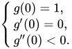 ${\begin{cases}g(0)=1,\\g'(0)=0,\\g''(0)<0.\end{cases}}$ For a particular form of solution with a quadratic dependence of the solution near x = 0, α = 2.5029... is one of the Feigenbaum constants.

The power series of $g$ is approximately $g(x)=1-1.52763x^{2}+0.104815x^{4}+0.026705x^{6}+O(x^{8})$

03Renormalization

The Feigenbaum function can be derived by a renormalization argument.

The Feigenbaum function satisfies $g(x)=\lim _{n\to \infty }{\frac {1}{F^{\left(2^{n}\right)}(0)}}F^{\left(2^{n}\right)}\left(xF^{\left(2^{n}\right)}(0)\right)$ for any map on the real line $F$ at the onset of chaos.

04Scaling function

The Feigenbaum scaling function provides a complete description of the attractor of the logistic map at the end of the period-doubling cascade. The attractor is a Cantor set, and just as the middle-third Cantor set, it can be covered by a finite set of segments, all bigger than a minimal size d_n. For a fixed d_n the set of segments forms a cover Δ_n of the attractor. The ratio of segments from two consecutive covers, Δ_n and Δ_n+1 can be arranged to approximate a function σ, the Feigenbaum scaling function.

Watch videos about Feigenbaum functionExplainers and documentaries on YouTube (opens in a new tab)

Sources and credits

This article is adapted from the Wikipedia article “Feigenbaum function”, written by its contributors and licensed under CC BY-SA 4.0. Fathomly has changed the layout, removed citation markers, navigation and maintenance notices, and adjusted punctuation. This adapted version is shared under the same license. For references, see the original article.

Images, from Wikimedia Commons:

Logistic iterates, together, r=3.56994567.svg by Cosmia Nebula, CC BY-SA 4.0
Logistic scaling limit, r=3.56994567.svg by Cosmia Nebula, CC BY-SA 4.0

Fathomly is not affiliated with or endorsed by the Wikimedia Foundation. Spotted a problem? Tell us.