Fast multipole method
Numerical technique
The fast multipole method (FMM) is a numerical technique that was developed to speed up the calculation of long-ranged forces in the n-body problem. It does this by expanding the system Green's function using a multipole expansion, which allows one to group sources that lie close together and treat them as if they were a single source.
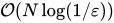
The FMM has also been applied in accelerating the iterative solver in the method of moments (MoM) as applied to computational electromagnetics problems, and in particular in computational bioelectromagnetism. The FMM was first introduced in this manner by Leslie Greengard and Vladimir Rokhlin Jr. and is based on the multipole expansion of the vector Helmholtz equation. By treating the interactions between far-away basis functions using the FMM, the corresponding matrix elements do not need to be explicitly stored, resulting in a significant reduction in required memory. If the FMM is then applied in a hierarchical manner, it can improve the complexity of matrix-vector products in an iterative solver from 


The FMM, introduced by Rokhlin Jr. and Greengard has been said to be one of the top ten algorithms of the 20th century. The FMM algorithm reduces the complexity of matrix-vector multiplication involving a certain type of dense matrix which can arise out of many physical systems.
The FMM has also been applied for efficiently treating the Coulomb interaction in the Hartree-Fock method and density functional theory calculations in quantum chemistry.
01Sketch of the algorithm
In its simplest form, the fast multipole method seeks to evaluate the following function:

![x_{\alpha }\in [-1,1]](https://wikimedia.org/api/rest_v1/media/math/render/svg/a185a37486af90479a8dbe37b4dbadf34d7db5f6)

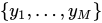
![y_{\beta }\in [-1,1]](https://wikimedia.org/api/rest_v1/media/math/render/svg/5e88504c64bfd9898b45526f92819699b82944df)

Naively, evaluating 





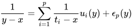


The speed-up of the fast multipole method derives from this interpolation: provided that all the poles are "far away", we evaluate the sum only on the Chebyshev nodes at a cost of 


Since 


To ensure that the poles are indeed well-separated, one recursively subdivides the unit interval such that only 


Sources and credits
This article is adapted from the Wikipedia article “Fast multipole method”, written by its contributors and licensed under CC BY-SA 4.0. Fathomly has changed the layout, removed citation markers, navigation and maintenance notices, and adjusted punctuation. This adapted version is shared under the same license. For references, see the original article.
Images, from Wikimedia Commons:
- Fast Multipoles - Local Expansion.svg by Summentier, CC BY-SA 4.0
Fathomly is not affiliated with or endorsed by the Wikimedia Foundation. Spotted a problem? Tell us.

