Encyclopedia

Explicit and implicit methods

Approaches for approximating solutions to differential equations

Wikipedia contributorsAdapted for Fathomly · View authors

3 min read
Source updated August 3, 2026

Explicit and implicit methods are approaches used in numerical analysis for obtaining numerical approximations to the solutions of ordinary and partial differential equations, as is required in computer simulations of physical processes. Explicit methods calculate the state of a system at a later time from the state of the system at the current time, while implicit methods find a solution by solving an equation involving both the current state of the system and the later one. Mathematically, if $Y(t)$ is the current system state and $Y(t+\Delta t)$ is the state at the later time ( $\Delta t$ is a small time step), then, for an explicit method

$Y(t+\Delta t)=F(Y(t))\,$

while for an implicit method one solves an equation

$G{\Big (}Y(t),Y(t+\Delta t){\Big )}=0\qquad (1)\,$

to find $Y(t+\Delta t).$

01Computation

Implicit methods require an extra computation (solving the above equation), and they can be much harder to implement. Implicit methods are used because many problems arising in practice are stiff, for which the use of an explicit method requires impractically small time steps $\Delta t$ to keep the error in the result bounded (see numerical stability). For such problems, to achieve given accuracy, it takes much less computational time to use an implicit method with larger time steps, even taking into account that one needs to solve an equation of the form (1) at each time step. That said, whether one should use an explicit or implicit method depends upon the problem to be solved.

Since the implicit method cannot be carried out for each kind of differential operator, it is sometimes advisable to make use of the so called operator splitting method, which means that the differential operator is rewritten as the sum of two complementary operators

$Y(t+\Delta t)=F(Y(t+\Delta t))+G(Y(t)),\,$

while one is treated explicitly and the other implicitly. For usual applications the implicit term is chosen to be linear while the explicit term can be nonlinear. This combination of the former method is called Implicit-Explicit Method (short IMEX,).

02Illustration using the forward and backward Euler methods

Consider the ordinary differential equation

${\frac {dy}{dt}}=-y^{2},\ t\in [0,a]\quad \quad (2)$

with the initial condition $y(0)=1.$ This problem has the exact solution $y={\frac {1}{t+1}}$ , which usually cannot be written down for problems encountered in practice, but in this case allows a comparison with the numerical solutions. Consider a grid $t_{k}=a{\frac {k}{n}}$ for 0 ≤ k ≤ n, that is, the time step is $\Delta t=a/n,$ and denote $y_{k}=y(t_{k})$ for each $k$ . Discretize this equation using the simplest explicit and implicit methods, which are the forward Euler and backward Euler methods (see numerical ordinary differential equations) and compare the obtained schemes.

Forward Euler method

The forward Euler method

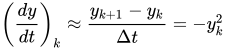
$\left({\frac {dy}{dt}}\right)_{k}\approx {\frac {y_{k+1}-y_{k}}{\Delta t}}=-y_{k}^{2}$

yields

$y_{k+1}=y_{k}-\Delta ty_{k}^{2}\quad \quad \quad (3)\,$

for each $k=0,1,\dots ,n.$ This is an explicit formula for $y_{k+1}$ .

Backward Euler method

With the backward Euler method

${\frac {y_{k+1}-y_{k}}{\Delta t}}=-y_{k+1}^{2}$

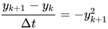
one finds the implicit equation

$y_{k+1}+\Delta ty_{k+1}^{2}=y_{k}$

for $y_{k+1}$ (compare this with formula (3) where $y_{k+1}$ was given explicitly rather than as an unknown in an equation).

This is a quadratic equation, having one negative and one positive root. The positive root is picked because in the original equation the initial condition is positive, and then $y$ at the next time step is given by

$y_{k+1}={\frac {-1+{\sqrt {1+4\Delta ty_{k}}}}{2\Delta t}}.\quad \quad (4)$

In the vast majority of cases, the equation to be solved when using an implicit scheme is much more complicated than a quadratic equation, and no analytical solution exists. Then one uses root-finding algorithms, such as Newton's method, to find the numerical solution.

Crank-Nicolson method

The Crank-Nicolson method, also known as the trapezoidal rule, can be thought of as an average of the forward and backward Euler methods. For the differential equation considered above, this gives

${\frac {y_{k+1}-y_{k}}{\Delta t}}=-{\frac {1}{2}}y_{k+1}^{2}-{\frac {1}{2}}y_{k}^{2}$

leading to the implicit equation

$y_{k+1}+{\frac {1}{2}}{\Delta t}y_{k+1}^{2}=y_{k}-{\frac {1}{2}}\Delta ty_{k}^{2}$

for $y_{k+1}$ (compare this with formula (3) where $y_{k+1}$ was given explicitly rather than as an unknown in an equation). This can be numerically solved using root-finding algorithms, such as Newton's method, to obtain $y_{k+1}$ .

The advantage of this method is its improved accuracy (see diagram above). Both Euler methods are first order, but the trapezoidal method is second order.

IMEX methods

Because of the difficulty of solving implicit equations, some methods use an implicit method for linear terms and an explicit method for nonlinear terms. These are called IMEX (Implicit-Explicit) schemes.

To illustrate the idea of IMEX schemes, consider a slightly different differential equation:

${\frac {dy}{dt}}=y-y^{2},\ t\in [0,a]\quad \quad (5)$

Using implicit Euler for the linear term and explicit Euler for the nonlinear term gives

${\frac {y_{k+1}-y_{k}}{\Delta t}}\approx y_{k+1}-y_{k}^{2},\ t\in [0,a].$

This equation is linear in $y_{k+1}$ so it can be solved to give

$y_{k+1}={\frac {y_{k}(1-y_{k}\Delta t)}{1-\Delta t}}\quad \quad (6)$

for each $k=0,1,\dots ,n.$ This method is sometimes called the Forward-Backward Euler method (see diagram).

Watch videos about Explicit and implicit methodsExplainers and documentaries on YouTube (opens in a new tab)

Sources and credits

This article is adapted from the Wikipedia article “Explicit and implicit methods”, written by its contributors and licensed under CC BY-SA 4.0. Fathomly has changed the layout, removed citation markers, navigation and maintenance notices, and adjusted punctuation. This adapted version is shared under the same license. For references, see the original article.

Images, from Wikimedia Commons:

Result of applying integration schemes.png by Jaiswal0, CC BY-SA 4.0
Comparison between Foward-Backward-Euler and Foward-Euler.png by Bug remains, CC0

Fathomly is not affiliated with or endorsed by the Wikimedia Foundation. Spotted a problem? Tell us.

Explicit and implicit methods

01Computation

02Illustration using the forward and backward Euler methods

Sources and credits

Related topics

Courant-Friedrichs-Lewy condition

SIMPLE algorithm