Exact diagonalization
Numerical technique for solving quantum Hamiltonians
Exact diagonalization (ED) is a numerical technique used in physics to determine the eigenstates and energy eigenvalues of a quantum Hamiltonian. In this technique, a Hamiltonian for a discrete, finite system is expressed in matrix form and diagonalized using a computer. Exact diagonalization is only feasible for systems with few degrees of freedom, due to the exponential growth of the Hilbert space dimension with the size of the quantum system. It is frequently employed to study lattice models, including the Hubbard model, Ising model, Heisenberg model, t-J model, and SYK model.
01Expectation values from exact diagonalization
After determining the eigenstates 


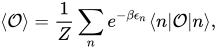
where 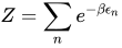
Green's functions may be evaluated similarly. For example, the retarded Green's function ![G^{R}(t)=-i\theta (t)\langle [A(t),B(0)]\rangle](https://wikimedia.org/api/rest_v1/media/math/render/svg/278fb263eacef0a3b1141b603b9a5d235fabcd4c)

Exact diagonalization can also be used to determine the time evolution of a system after a quench. Suppose the system has been prepared in an initial state 



02Memory requirements
The dimension of the Hilbert space describing a quantum system scales exponentially with system size. For example, consider a system of 


| Number of sites | Number of states | Hamiltonian size in memory |
|---|---|---|
| 4 | 16 | 2048 B |
| 9 | 512 | 2 MB |
| 16 | 65536 | 34 GB |
| 25 | 33554432 | 9 PB |
| 36 | 6.872e10 | 40 ZB |
03Comparison with other techniques
Exact diagonalization is useful for extracting exact information about finite systems. However, often small systems are studied to gain insight into infinite lattice systems. If the diagonalized system is too small, its properties will not reflect the properties of the system in the thermodynamic limit, and the simulation is said to suffer from finite size effects.
Unlike some other exact theory techniques, such as Auxiliary-field Monte Carlo, exact diagonalization obtains Green's functions directly in real time, as opposed to imaginary time. Unlike in these other techniques, exact diagonalization results do not need to be numerically analytically continued. This is an advantage, because numerical analytic continuation is an ill-posed and difficult optimization problem.
04Applications
- Can be used as an impurity solver for Dynamical mean-field theory techniques.
- When combined with finite size scaling, estimating the ground state energy and critical exponents of the 1D transverse-field Ising model.
- Studying properties of the 2D Heisenberg model in a magnetic field, including antiferromagnetism and spin-wave velocity.
- Studying the Drude weight of the 2D Hubbard model.
- Studying out-of-time-order correlations (OTOCs) and scrambling in the SYK model.
- Simulating resonant x-ray spectra of strongly correlated materials.
- Simulating the nonlinear spectroscopy of quantum magnets.
05Implementations
06Generalizations
Exact diagonalization results from many small clusters can be combined to obtain more accurate information about systems in the thermodynamic limit using the numerical linked cluster expansion.
Sources and credits
This article is adapted from the Wikipedia article “Exact diagonalization”, written by its contributors and licensed under CC BY-SA 4.0. Fathomly has changed the layout, removed citation markers, navigation and maintenance notices, and adjusted punctuation. This adapted version is shared under the same license. For references, see the original article.
Fathomly is not affiliated with or endorsed by the Wikimedia Foundation. Spotted a problem? Tell us.