Encyclopedia

Probability space

Mathematical concept

Wikipedia contributorsAdapted for Fathomly · View authors

11 min read
Source updated June 11, 2026

In probability theory, a probability space or a probability triple $(\Omega ,{\mathcal {F}},P)$ is a mathematical construct that provides a formal model of a random process or experiment.

A probability space consists of three elements:

A sample space, $\Omega$ , which is the set of all possible outcomes of a random process under consideration.
An event space, ${\mathcal {F}}$ , which is a set of events, where an event is a subset of outcomes in the sample space.
A probability function, $P$ , which assigns, to each event in the event space, a probability, which is a number between 0 and 1 (inclusive).

In order to provide a model of probability, these elements must satisfy probability axioms.

For example, one can define a probability space which models the throwing of a dice:

The sample space $\Omega$ is typically the set $\{1,2,3,4,5,6\}$ where each element in the set is a label which represents the outcome of the die landing on that label. For example, $1$ represents the outcome that the die lands on 1.
The event space ${\mathcal {F}}$ could be the set of all subsets of the sample space, which would then contain simple events such as $\{5\}$ ("the die lands on 5"), as well as complex events such as $\{2,4,6\}$ ("the die lands on an even number").
The probability function $P$ would then map each event to the number of outcomes in that event divided by 6, so for example, $\{5\}$ would be mapped to $1/6$ , and $\{2,4,6\}$ would be mapped to $3/6=1/2$ .

When an experiment is conducted, it results in exactly one outcome $\omega$ from the sample space $\Omega$ . All the events in the event space ${\mathcal {F}}$ that contain the selected outcome $\omega$ are said to "have occurred". The probability function $P$ must be so defined that if the experiment were repeated arbitrarily many times, the number of occurrences of each event as a fraction of the total number of experiments, will most likely tend towards the probability assigned to that event.

The Soviet mathematician Andrey Kolmogorov introduced the notion of a probability space and the axioms of probability in the 1930s. In modern probability theory, there are alternative approaches for axiomatization, such as the algebra of random variables.

01Introduction

A probability space is a mathematical triplet $(\Omega ,{\mathcal {F}},P)$ that presents a model for a particular class of real-world situations. As with other models, its author ultimately defines which elements $\Omega$ , ${\mathcal {F}}$ , and $P$ will contain.

The sample space $\Omega$ is the set of all possible outcomes. An outcome is the result of a single execution of the model. Outcomes may be states of nature, possibilities, experimental results and the like. Every instance of the real-world situation (or run of the experiment) must produce exactly one outcome. If outcomes of different runs of an experiment differ in any way that matters, they are distinct outcomes. Which differences matter depends on the kind of analysis we want to do. This leads to different choices of sample space.
The σ-algebra ${\mathcal {F}}$ is a collection of all the events we would like to consider. This collection may or may not include each of the elementary events. Here, an "event" is a set of zero or more outcomes; that is, a subset of the sample space. An event is considered to have "happened" during an experiment when the outcome of the latter is an element of the event. Since the same outcome may be a member of many events, it is possible for many events to have happened given a single outcome. For example, when the trial consists of throwing two dice, the set of all outcomes with a sum of 7 pips may constitute an event, whereas outcomes with an odd number of pips may constitute another event. If the outcome is the element of the elementary event of two pips on the first die and five on the second, then both of the events, "7 pips" and "odd number of pips", are said to have happened.
The probability measure $P$ is a set function returning an event's probability. A probability is a real number between zero (impossible events have probability zero, though probability-zero events are not necessarily impossible) and one (the event happens almost surely, with almost total certainty). Thus $P$ is a function $P:{\mathcal {F}}\to [0,1].$ The probability measure function must satisfy two simple requirements: First, the probability of a countable union of mutually exclusive events must be equal to the countable sum of the probabilities of each of these events. For example, the probability of the union of the mutually exclusive events ${\text{Head}}$ and ${\text{Tail}}$ in the random experiment of one coin toss, $P({\text{Head}}\cup {\text{Tail}})$ , is the sum of probability for ${\text{Head}}$ and the probability for ${\text{Tail}}$ , $P({\text{Head}})+P({\text{Tail}})$ . Second, the probability of the sample space $\Omega$ must be equal to 1 (which accounts for the fact that, given an execution of the model, some outcome must occur). In the previous example the probability of the set of outcomes $P(\{{\text{Head}},{\text{Tail}}\})$ must be equal to one, because it is entirely certain that the outcome will be either ${\text{Head}}$ or ${\text{Tail}}$ (the model neglects any other possibility) in a single coin toss.

Not every subset of the sample space $\Omega$ must necessarily be considered an event: some of the subsets are simply not of interest, others cannot be "measured". This is not so obvious in a case like a coin toss. In a different example, one could consider javelin throw lengths, where the events typically are intervals like "between 60 and 65 meters" and unions of such intervals, but not sets like the "irrational numbers between 60 and 65 meters".

02Definition

In short, a probability space is a measure space such that the measure of the whole space is equal to one.

The expanded definition is the following: a probability space is a triple $(\Omega ,{\mathcal {F}},P)$ consisting of:

the sample space $\Omega$ , an arbitrary non-empty set,
the σ-algebra (also called σ-field), a set of subsets of , called events, such that:
- ${\mathcal {F}}$ contains the sample space: $\Omega \in {\mathcal {F}}$ ,
- ${\mathcal {F}}$ is closed under complements: if $A\in {\mathcal {F}}$ , then also $(\Omega \setminus A)\in {\mathcal {F}}$ ,
- is closed under countable unions: if for , then also
  - The corollary from the previous two properties and De Morgan's law is that ${\mathcal {F}}$ is also closed under countable intersections: if $A_{i}\in {\mathcal {F}}$ for $i=1,2,\dots$ , then also ${\textstyle (\bigcap _{i=1}^{\infty }A_{i})\in {\mathcal {F}}$
the probability measure , a function on such that:
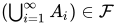
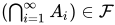
- P is countably additive (also called σ-additive): if $\{A_{i}\}_{i=1}^{\infty }\subseteq {\mathcal {F}}$ is a countable collection of pairwise disjoint sets, then ${\textstyle P(\bigcup _{i=1}^{\infty }A_{i})=\sum _{i=1}^{\infty }P(A_{i}),$
- the measure of the entire sample space is equal to one: $P(\Omega )=1$ .

03Discrete case

For a countable sample space $\Omega$ , probabilities can be ascribed to elements of $\Omega$ by a discrete probability distribution $p:\Omega \to [0,1]$ such that ${\textstyle \sum _{\omega \in \Omega }p(\omega )=1,$ whereby all subsets of $\Omega$ can be treated as events (thus, ${\mathcal {F}}=2^{\Omega }$ is the power set) and the probability measure has the form

P(A)=\sum _{\omega \in A}p(\omega )\quad {\text{for all }}A\subseteq \Omega .

The greatest σ-algebra ${\mathcal {F}}=2^{\Omega }$ describes the complete information. In general, a σ-algebra ${\mathcal {F}}\subseteq 2^{\Omega }$ corresponds to a finite or countable partition $\Omega =B_{1}\cup B_{2}\cup \dots$ , the general form of an event $A\in {\mathcal {F}}$ being $A=B_{k_{1}}\cup B_{k_{2}}\cup \dots$ .

The case $p(\omega )=0$ is permitted by the definition, but rarely used, since such $\omega$ can safely be excluded from the sample space.

04General case

If Ω is uncountable, still, it may happen that P(ω) ≠ 0 for some ω; such ω are called atoms. They are an at most countable (maybe empty) set, whose probability is the sum of probabilities of all atoms. If this sum is equal to 1 then all other points can safely be excluded from the sample space, returning us to the discrete case. Otherwise, if the sum of probabilities of all atoms is between 0 and 1, then the probability space decomposes into a discrete (atomic) part (maybe empty) and a non-atomic part.

05Non-atomic case

If P(ω) = 0 for all ω ∈ Ω, then Ω must be uncountable (otherwise the axiom P(Ω) = 1 would be rendered impossible) and equation (1) does not apply: the probability of a set is not necessarily the sum over the probabilities of its elements, as summation is only defined for countable numbers of elements. This makes the probability space theory much more technical. A formulation stronger than summation, measure theory is applicable. Initially the probabilities are ascribed to some "generator" sets (see the examples). Then a limiting procedure allows assigning probabilities to sets that are limits of sequences of generator sets, or limits of limits, and so on. All these sets are the σ-algebra ${\mathcal {F}}$ . For technical details see Carathéodory's extension theorem. Sets belonging to ${\mathcal {F}}$ are called measurable. In general they are much more complicated than generator sets, but much better than non-measurable sets.

06Complete probability space

A probability space $(\Omega ,\;{\mathcal {F}},\;P)$ is said to be a complete probability space if for all $B\in {\mathcal {F}}$ with $P(B)=0$ and all $A\;\subset \;B$ one has $A\in {\mathcal {F}}$ . Often, the study of probability spaces is restricted to complete probability spaces.

07Examples

Discrete examples

Example 1

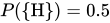
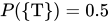
If the experiment consists of just one flip of a fair coin, then the outcome is either heads or tails: $\Omega =\{{\text{H}},{\text{T}}\}$ . The σ-algebra ${\mathcal {F}}=2^{\Omega }$ contains $2^{2}=4$ events, namely: $\{{\text{H}}\}$ ("heads"), $\{{\text{T}}\}$ ("tails"), $\{\}$ ("neither heads nor tails"), and $\{{\text{H}},{\text{T}}\}$ ("either heads or tails"); in other words, ${\mathcal {F}}=\{\{\},\{{\text{H}}\},\{{\text{T}}\},\{{\text{H}},{\text{T}}\}\}$ . There is a fifty percent chance of tossing heads and fifty percent for tails, so the probability measure in this example is $P(\{\})=0$ , $P(\{{\text{H}}\})=0.5$ , $P(\{{\text{T}}\})=0.5$ , $P(\{{\text{H}},{\text{T}}\})=1$ .

Example 2

The fair coin is tossed three times. There are 8 possible outcomes: Ω = {HHH, HHT, HTH, HTT, THH, THT, TTH, TTT} (here "HTH" for example means that first time the coin landed heads, the second time tails, and the last time heads again). The complete information is described by the σ-algebra ${\mathcal {F}}=2^{\Omega }$ of 2⁸ = 256 events, where each of the events is a subset of Ω.

Alice knows the outcome of the second toss only. Thus her incomplete information is described by the partition Ω = A₁ ⊔ A₂ = {HHH, HHT, THH, THT} ⊔ {HTH, HTT, TTH, TTT}, where ⊔ is the disjoint union, and the corresponding σ-algebra ${\mathcal {F}}_{\text{Alice}}=\{\{\},A_{1},A_{2},\Omega \}$ . Bryan knows only the total number of tails. His partition contains four parts: Ω = B₀ ⊔ B₁ ⊔ B₂ ⊔ B₃ = {HHH} ⊔ {HHT, HTH, THH} ⊔ {TTH, THT, HTT} ⊔ {TTT}; accordingly, his σ-algebra ${\mathcal {F}}_{\text{Bryan}}$ contains 2⁴ = 16 events.

The two σ-algebras are incomparable: neither ${\mathcal {F}}_{\text{Alice}}\subseteq {\mathcal {F}}_{\text{Bryan}}$ nor ${\mathcal {F}}_{\text{Bryan}}\subseteq {\mathcal {F}}_{\text{Alice}}$ ; both are sub-σ-algebras of 2^Ω.

Example 3

If 100 voters are to be drawn randomly from among all voters in California and asked whom they will vote for governor, then the set of all sequences of 100 Californian voters would be the sample space Ω. We assume that sampling without replacement is used: only sequences of 100 different voters are allowed. For simplicity an ordered sample is considered, that is a sequence (Alice, Bryan) is different from (Bryan, Alice). We also take for granted that each potential voter knows exactly his/her future choice, that is he/she does not choose randomly.

Alice knows only whether or not Arnold Schwarzenegger has received at least 60 votes. Her incomplete information is described by the σ-algebra ${\mathcal {F}}_{\text{Alice}}$ that contains: (1) the set of all sequences in Ω where at least 60 people vote for Schwarzenegger; (2) the set of all sequences where fewer than 60 vote for Schwarzenegger; (3) the whole sample space Ω; and (4) the empty set ∅.

Bryan knows the exact number of voters who are going to vote for Schwarzenegger. His incomplete information is described by the corresponding partition Ω = B₀ ⊔ B₁ ⊔ ⋯ ⊔ B₁₀₀ and the σ-algebra ${\mathcal {F}}_{\text{Bryan}}$ consists of 2¹⁰¹ events.

In this case, Alice's σ-algebra is a subset of Bryan's: ${\mathcal {F}}_{\text{Alice}}\subset {\mathcal {F}}_{\text{Bryan}}$ . Bryan's σ-algebra is in turn a subset of the much larger "complete information" σ-algebra 2^Ω consisting of 2^{n(n−1)⋯(n−99)} events, where n is the number of all potential voters in California.

Non-atomic examples

Example 4

A number between 0 and 1 is chosen at random, uniformly. Here Ω = [0,1], ${\mathcal {F}}$ is the σ-algebra of Borel sets on Ω, and P is the Lebesgue measure on [0,1].

In this case, the open intervals of the form (a,b), where 0 < a < b < 1, could be taken as the generator sets. Each such set can be ascribed the probability of P((a,b)) = (b − a), which generates the Lebesgue measure on [0,1], and the Borel σ-algebra on Ω.

Example 5

A fair coin is tossed endlessly. Here one can take Ω = {0,1}^∞, the set of all infinite sequences of numbers 0 and 1. Cylinder sets {(x₁, x₂, ...) ∈ Ω : x₁ = a₁, ..., x_n = a_n} may be used as the generator sets. Each such set describes an event in which the first n tosses have resulted in a fixed sequence (a₁, ..., a_n), and the rest of the sequence may be arbitrary. Each such event can be naturally given the probability of 2⁻ⁿ.

These two non-atomic examples are closely related: a sequence (x₁, x₂, ...) ∈ {0,1}^∞ leads to the number 2⁻¹x₁ + 2⁻²x₂ + ⋯ ∈ [0,1]. This is not a one-to-one correspondence between {0,1}^∞ and [0,1] however: it is an isomorphism modulo zero, which allows for treating the two probability spaces as two forms of the same probability space. In fact, all non-pathological non-atomic probability spaces are the same in this sense. They are so-called standard probability spaces. Basic applications of probability spaces are insensitive to standardness. However, non-discrete conditioning is easy and natural on standard probability spaces, otherwise it becomes obscure.

08Related concepts

Probability distribution

Random variables

A random variable X is a measurable function X: Ω → S from the sample space Ω to another measurable space S called the state space.

If A ⊂ S, the notation Pr(X ∈ A) is a commonly used shorthand for $P(\{\omega \in \Omega :X(\omega )\in A\})$ .

Defining the events in terms of the sample space

If Ω is countable, we almost always define ${\mathcal {F}}$ as the power set of Ω, i.e. ${\mathcal {F}}=2^{\Omega }$ which is trivially a σ-algebra and the biggest one we can create using Ω. We can therefore omit ${\mathcal {F}}$ and just write (Ω,P) to define the probability space.

On the other hand, if Ω is uncountable and we use ${\mathcal {F}}=2^{\Omega }$ we get into trouble defining our probability measure P because ${\mathcal {F}}$ is too "large", i.e. there will often be sets to which it will be impossible to assign a unique measure. In this case, we have to use a smaller σ-algebra ${\mathcal {F}}$ , for example the Borel algebra of Ω, which is the smallest σ-algebra that makes all open sets measurable.

Conditional probability

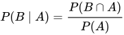
Kolmogorov's definition of probability spaces gives rise to the natural concept of conditional probability. Every set A with non-zero probability (that is, P(A) > 0) defines another probability measure $P(B\mid A)={P(B\cap A) \over P(A)}$ on the space. This is usually pronounced as the "probability of B given A".

For any event A such that P(A) > 0, the function Q defined by Q(B) = P(B | A) for all events B is itself a probability measure.

Independence

Two events, A and B are said to be independent if P(A ∩ B) = P(A) P(B).

Two random variables, X and Y, are said to be independent if any event defined in terms of X is independent of any event defined in terms of Y. Formally, they generate independent σ-algebras, where two σ-algebras G and H, which are subsets of F are said to be independent if any element of G is independent of any element of H.

Mutual exclusivity

Two events, A and B are said to be mutually exclusive or disjoint if the occurrence of one implies the non-occurrence of the other, i.e., their intersection is empty. This is a stronger condition than the probability of their intersection being zero.

If A and B are disjoint events, then P(A ∪ B) = P(A) + P(B). This extends to a (finite or countably infinite) sequence of events. However, the probability of the union of an uncountable set of events is not the sum of their probabilities. For example, if Z is a normally distributed random variable, then P(Z = x) is 0 for any x, but P(Z ∈ R) = 1.

The event A ∩ B is referred to as "A and B", and the event A ∪ B as "A or B".

Watch videos about Probability spaceExplainers and documentaries on YouTube (opens in a new tab)

Sources and credits

This article is adapted from the Wikipedia article “Probability space”, written by its contributors and licensed under CC BY-SA 4.0. Fathomly has changed the layout, removed citation markers, navigation and maintenance notices, and adjusted punctuation. This adapted version is shared under the same license. For references, see the original article.

Images, from Wikimedia Commons:

Standard deviation diagram micro.svg by Ainali, CC BY-SA 3.0
Dice measure.svg by Sascha Lill 95, CC BY-SA 4.0

Fathomly is not affiliated with or endorsed by the Wikimedia Foundation. Spotted a problem? Tell us.