Encyclopedia

Divided differences

Algorithm for computing polynomial coefficients

Wikipedia contributorsAdapted for Fathomly · View authors

3 min read
Source updated March 24, 2026

In mathematics, divided differences is an algorithm, historically used for computing tables of logarithms and trigonometric functions. Charles Babbage's difference engine, an early mechanical calculator, was designed to use this algorithm in its operation.

Divided differences is a recursive division process. Given a sequence of data points $(x_{0},y_{0}),\ldots ,(x_{n},y_{n})$ , the method calculates the coefficients of the interpolation polynomial of these points in the Newton form.

It is sometimes denoted by a delta with a bar: ${\text{△}}\!\!\!|\,\,$ or ${\text{◿}}\!{\text{◺}}$ .

01Definition

Given n + 1 data points $(x_{0},y_{0}),\ldots ,(x_{n},y_{n})$ where the $x_{k}$ are assumed to be pairwise distinct, the forward divided differences are defined as: ${\begin{aligned}{\mathopen {[}}y_{k}]&:=y_{k},&&k\in \{0,\ldots ,n\}\\{\mathopen {[}}y_{k},\ldots ,y_{j}]&:={\frac {[y_{k+1},\ldots ,y_{j}]-[y_{k},\ldots ,y_{j-1}]}{x_{j}-x_{k}}},&&k\in \{0,\ldots ,n-1\},\ j\in \{k+1,\ldots ,n\}.\end{aligned}}$

To make the recursive process of computation clearer, the divided differences can be put in tabular form, where the columns correspond to the value of j above, and each entry in the table is computed from the difference of the entries to its immediate lower left and to its immediate upper left, divided by a difference of corresponding x-values: ${\begin{matrix}x_{0}&y_{0}=[y_{0}]&&&\\&&[y_{0},y_{1}]&&\\x_{1}&y_{1}=[y_{1}]&&[y_{0},y_{1},y_{2}]&\\&&[y_{1},y_{2}]&&[y_{0},y_{1},y_{2},y_{3}]\\x_{2}&y_{2}=[y_{2}]&&[y_{1},y_{2},y_{3}]&\\&&[y_{2},y_{3}]&&\\x_{3}&y_{3}=[y_{3}]&&&\\\end{matrix}}$

Notation

Note that the divided difference $[y_{k},\ldots ,y_{k+j}]$ depends on the values $x_{k},\ldots ,x_{k+j}$ and $y_{k},\ldots ,y_{k+j}$ , but the notation hides the dependency on the x-values. If the data points are given by a function f, $(x_{0},y_{0}),\ldots ,(x_{k},y_{n})=(x_{0},f(x_{0})),\ldots ,(x_{n},f(x_{n}))$ one sometimes writes the divided difference in the notation $f[x_{k},\ldots ,x_{k+j}]\ {\stackrel {\text{def}}{=}}\ [f(x_{k}),\ldots ,f(x_{k+j})]=[y_{k},\ldots ,y_{k+j}].$ Other notations for the divided difference of the function ƒ on the nodes x₀, ..., x_n are: $f[x_{k},\ldots ,x_{k+j}]={\mathopen {[}}x_{0},\ldots ,x_{n}]f={\mathopen {[}}x_{0},\ldots ,x_{n};f]=D[x_{0},\ldots ,x_{n}]f.$

02Example

Divided differences for $k=0$ and the first few values of $j$ : ${\begin{aligned}{\mathopen {[}}y_{0}]&=y_{0}\\{\mathopen {[}}y_{0},y_{1}]&={\frac {y_{1}-y_{0}}{x_{1}-x_{0}}}\\{\mathopen {[}}y_{0},y_{1},y_{2}]&={\frac {{\mathopen {[}}y_{1},y_{2}]-{\mathopen {[}}y_{0},y_{1}]}{x_{2}-x_{0}}}={\frac {{\frac {y_{2}-y_{1}}{x_{2}-x_{1}}}-{\frac {y_{1}-y_{0}}{x_{1}-x_{0}}}}{x_{2}-x_{0}}}={\frac {y_{2}-y_{1}}{(x_{2}-x_{1})(x_{2}-x_{0})}}-{\frac {y_{1}-y_{0}}{(x_{1}-x_{0})(x_{2}-x_{0})}}\\{\mathopen {[}}y_{0},y_{1},y_{2},y_{3}]&={\frac {{\mathopen {[}}y_{1},y_{2},y_{3}]-{\mathopen {[}}y_{0},y_{1},y_{2}]}{x_{3}-x_{0}}}\end{aligned}}$

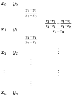
Thus, the table corresponding to these terms up to two columns has the following form: ${\begin{matrix}x_{0}&y_{0}&&\\&&{y_{1}-y_{0} \over x_{1}-x_{0}}&\\x_{1}&y_{1}&&{{y_{2}-y_{1} \over x_{2}-x_{1}}-{y_{1}-y_{0} \over x_{1}-x_{0}} \over x_{2}-x_{0}}\\&&{y_{2}-y_{1} \over x_{2}-x_{1}}&\\x_{2}&y_{2}&&\vdots \\&&\vdots &\\\vdots &&&\vdots \\&&\vdots &\\x_{n}&y_{n}&&\\\end{matrix}}$

03Properties

Linearity ${\begin{aligned}(f+g)[x_{0},\dots ,x_{n}]&=f[x_{0},\dots ,x_{n}]+g[x_{0},\dots ,x_{n}]\\(\lambda \cdot f)[x_{0},\dots ,x_{n}]&=\lambda \cdot f[x_{0},\dots ,x_{n}]\end{aligned}}$
Leibniz rule $(f\cdot g)[x_{0},\dots ,x_{n}]=f[x_{0}]\cdot g[x_{0},\dots ,x_{n}]+f[x_{0},x_{1}]\cdot g[x_{1},\dots ,x_{n}]+\dots +f[x_{0},\dots ,x_{n}]\cdot g[x_{n}]=\sum _{r=0}^{n}f[x_{0},\ldots ,x_{r}]\cdot g[x_{r},\ldots ,x_{n}]$
Divided differences are symmetric: If $\sigma :\{0,\dots ,n\}\to \{0,\dots ,n\}$ is a permutation then $f[x_{0},\dots ,x_{n}]=f[x_{\sigma (0)},\dots ,x_{\sigma (n)}]$
Polynomial interpolation in the Newton form: if $P$ is a polynomial function of degree $\leq n$ , and $p[x_{0},\dots ,x_{n}]$ is the divided difference, then $P_{n-1}(x)=p[x_{0}]+p[x_{0},x_{1}](x-x_{0})+p[x_{0},x_{1},x_{2}](x-x_{0})(x-x_{1})+\cdots +p[x_{0},\ldots ,x_{n}](x-x_{0})(x-x_{1})\cdots (x-x_{n-1})$
If $p$ is a polynomial function of degree $<n$ , then $p[x_{0},\dots ,x_{n}]=0.$
Mean value theorem for divided differences: if $f$ is n times differentiable, then $f[x_{0},\dots ,x_{n}]={\frac {f^{(n)}(\xi )}{n!}}$ for a number $\xi$ in the open interval determined by the smallest and largest of the $x_{k}$ 's.

04Matrix form

The divided difference scheme can be put into an upper triangular matrix: $T_{f}(x_{0},\dots ,x_{n})={\begin{pmatrix}f[x_{0}]&f[x_{0},x_{1}]&f[x_{0},x_{1},x_{2}]&\ldots &f[x_{0},\dots ,x_{n}]\\0&f[x_{1}]&f[x_{1},x_{2}]&\ldots &f[x_{1},\dots ,x_{n}]\\0&0&f[x_{2}]&\ldots &f[x_{2},\dots ,x_{n}]\\\vdots &\vdots &&\ddots &\vdots \\0&0&0&\ldots &f[x_{n}]\end{pmatrix}}.$

Then it holds

$T_{f+g}(x)=T_{f}(x)+T_{g}(x)$
$T_{\lambda f}(x)=\lambda T_{f}(x)$ if $\lambda$ is a scalar
$T_{f\cdot g}(x)=T_{f}(x)\cdot T_{g}(x)$

This follows from the Leibniz rule. It means that multiplication of such matrices is commutative. Summarised, the matrices of divided difference schemes with respect to the same set of nodes x form a commutative ring.
Since $T_{f}(x)$ is a triangular matrix, its eigenvalues are obviously $f(x_{0}),\dots ,f(x_{n})$ .
Let $\delta _{\xi }$ be a Kronecker delta-like function, that is $\delta _{\xi }(t)={\begin{cases}1&:t=\xi ,\\0&:{\mbox{else}}.\end{cases}}$ Obviously $f\cdot \delta _{\xi }=f(\xi )\cdot \delta _{\xi }$ , thus $\delta _{\xi }$ is an eigenfunction of the pointwise function multiplication. That is $T_{\delta _{x_{i}}}(x)$ is somehow an "eigenmatrix" of $T_{f}(x)$ : $T_{f}(x)\cdot T_{\delta _{x_{i}}}(x)=f(x_{i})\cdot T_{\delta _{x_{i}}}(x)$ . However, all columns of $T_{\delta _{x_{i}}}(x)$ are multiples of each other, the matrix rank of $T_{\delta _{x_{i}}}(x)$ is 1. So you can compose the matrix of all eigenvectors of $T_{f}(x)$ from the $i$ -th column of each $T_{\delta _{x_{i}}}(x)$ . Denote the matrix of eigenvectors with $U(x)$ . Example $U(x_{0},x_{1},x_{2},x_{3})={\begin{pmatrix}1&{\frac {1}{(x_{1}-x_{0})}}&{\frac {1}{(x_{2}-x_{0})(x_{2}-x_{1})}}&{\frac {1}{(x_{3}-x_{0})(x_{3}-x_{1})(x_{3}-x_{2})}}\\0&1&{\frac {1}{(x_{2}-x_{1})}}&{\frac {1}{(x_{3}-x_{1})(x_{3}-x_{2})}}\\0&0&1&{\frac {1}{(x_{3}-x_{2})}}\\0&0&0&1\end{pmatrix}}$ The diagonalization of $T_{f}(x)$ can be written as $U(x)\cdot \operatorname {diag} (f(x_{0}),\dots ,f(x_{n}))=T_{f}(x)\cdot U(x).$

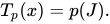
Polynomials and power series

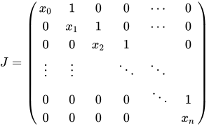
The matrix $J={\begin{pmatrix}x_{0}&1&0&0&\cdots &0\\0&x_{1}&1&0&\cdots &0\\0&0&x_{2}&1&&0\\\vdots &\vdots &&\ddots &\ddots &\\0&0&0&0&\;\ddots &1\\0&0&0&0&&x_{n}\end{pmatrix}}$ contains the divided difference scheme for the identity function with respect to the nodes $x_{0},\dots ,x_{n}$ , thus $J^{m}$ contains the divided differences for the power function with exponent $m$ . Consequently, you can obtain the divided differences for a polynomial function $p$ by applying $p$ to the matrix $J$ : If $p(\xi )=a_{0}+a_{1}\cdot \xi +\dots +a_{m}\cdot \xi ^{m}$ and $p(J)=a_{0}+a_{1}\cdot J+\dots +a_{m}\cdot J^{m}$ then $T_{p}(x)=p(J).$ This is known as Opitz' formula.

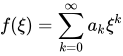
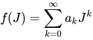
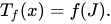
Now consider increasing the degree of $p$ to infinity, i.e. turn the Taylor polynomial into a Taylor series. Let $f$ be a function which corresponds to a power series. You can compute the divided difference scheme for $f$ by applying the corresponding matrix series to $J$ : If $f(\xi )=\sum _{k=0}^{\infty }a_{k}\xi ^{k}$ and $f(J)=\sum _{k=0}^{\infty }a_{k}J^{k}$ then $T_{f}(x)=f(J).$

05Alternative characterizations

Expanded form

${\begin{aligned}f[x_{0}]&=f(x_{0})\\f[x_{0},x_{1}]&={\frac {f(x_{0})}{(x_{0}-x_{1})}}+{\frac {f(x_{1})}{(x_{1}-x_{0})}}\\f[x_{0},x_{1},x_{2}]&={\frac {f(x_{0})}{(x_{0}-x_{1})\cdot (x_{0}-x_{2})}}+{\frac {f(x_{1})}{(x_{1}-x_{0})\cdot (x_{1}-x_{2})}}+{\frac {f(x_{2})}{(x_{2}-x_{0})\cdot (x_{2}-x_{1})}}\\f[x_{0},x_{1},x_{2},x_{3}]&={\frac {f(x_{0})}{(x_{0}-x_{1})\cdot (x_{0}-x_{2})\cdot (x_{0}-x_{3})}}+{\frac {f(x_{1})}{(x_{1}-x_{0})\cdot (x_{1}-x_{2})\cdot (x_{1}-x_{3})}}+\\&\quad \quad {\frac {f(x_{2})}{(x_{2}-x_{0})\cdot (x_{2}-x_{1})\cdot (x_{2}-x_{3})}}+{\frac {f(x_{3})}{(x_{3}-x_{0})\cdot (x_{3}-x_{1})\cdot (x_{3}-x_{2})}}\\f[x_{0},\dots ,x_{n}]&=\sum _{j=0}^{n}{\frac {f(x_{j})}{\prod _{k\in \{0,\dots ,n\}\setminus \{j\}}(x_{j}-x_{k})}}\end{aligned}}$

With the help of the polynomial function $\omega (\xi )=(\xi -x_{0})\cdots (\xi -x_{n})$ this can be written as $f[x_{0},\dots ,x_{n}]=\sum _{j=0}^{n}{\frac {f(x_{j})}{\omega '(x_{j})}}.$

Peano form

If $x_{0}<x_{1}<\cdots <x_{n}$ and $n\geq 1$ , the divided differences can be expressed as $f[x_{0},\ldots ,x_{n}]={\frac {1}{(n-1)!}}\int _{x_{0}}^{x_{n}}f^{(n)}(t)\;B_{n-1}(t)\,dt$ where $f^{(n)}$ is the $n$ -th derivative of the function $f$ and $B_{n-1}$ is a certain B-spline of degree $n-1$ for the data points $x_{0},\dots ,x_{n}$ , given by the formula $B_{n-1}(t)=\sum _{k=0}^{n}{\frac {(\max(0,x_{k}-t))^{n-1}}{\omega '(x_{k})}}$

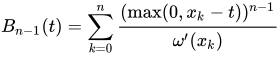
This is a consequence of the Peano kernel theorem; it is called the Peano form of the divided differences and $B_{n-1}$ is the Peano kernel for the divided differences, all named after Giuseppe Peano.

Forward and backward differences

When the data points are equidistantly distributed we get the special case called forward differences. They are easier to calculate than the more general divided differences.

Given n+1 data points $(x_{0},y_{0}),\ldots ,(x_{n},y_{n})$ with $x_{k}=x_{0}+kh,\ {\text{ for }}\ k=0,\ldots ,n{\text{ and fixed }}h>0$ the forward differences are defined as: ${\begin{aligned}\Delta ^{(0)}y_{k}&:=y_{k},\qquad k=0,\ldots ,n\\\Delta ^{(j)}y_{k}&:=\Delta ^{(j-1)}y_{k+1}-\Delta ^{(j-1)}y_{k},\qquad k=0,\ldots ,n-j,\ j=1,\dots ,n.\end{aligned}}$
whereas the backward differences are defined as: ${\begin{aligned}\nabla ^{(0)}y_{k}&:=y_{k},\qquad k=0,\ldots ,n\\\nabla ^{(j)}y_{k}&:=\nabla ^{(j-1)}y_{k}-\nabla ^{(j-1)}y_{k-1},\qquad k=0,\ldots ,n-j,\ j=1,\dots ,n.\end{aligned}}$
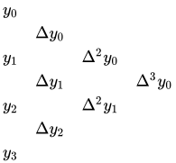
Thus the forward difference table is written as: ${\begin{matrix}y_{0}&&&\\&\Delta y_{0}&&\\y_{1}&&\Delta ^{2}y_{0}&\\&\Delta y_{1}&&\Delta ^{3}y_{0}\\y_{2}&&\Delta ^{2}y_{1}&\\&\Delta y_{2}&&\\y_{3}&&&\\\end{matrix}}$
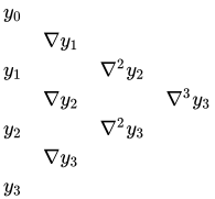
whereas the backwards difference table is written as: ${\begin{matrix}y_{0}&&&\\&\nabla y_{1}&&\\y_{1}&&\nabla ^{2}y_{2}&\\&\nabla y_{2}&&\nabla ^{3}y_{3}\\y_{2}&&\nabla ^{2}y_{3}&\\&\nabla y_{3}&&\\y_{3}&&&\\\end{matrix}}$

The relationship between divided differences and forward differences is $[y_{j},y_{j+1},\ldots ,y_{j+k}]={\frac {1}{k!h^{k}}}\Delta ^{(k)}y_{j},$ whereas for backward differences: $[{y}_{j},y_{j-1},\ldots ,{y}_{j-k}]={\frac {1}{k!h^{k}}}\nabla ^{(k)}y_{j}.$

Explicit formula

When the data points are equispaced we can also derive an explicit formula for $[y_{j},\ldots ,y_{j+k}]$ . For any fixed $k\leq n$ and $j$ such that $j+k\leq n$ , $[y_{j},\ldots ,y_{j+k}]={\frac {(-1)^{j+k}}{k!h^{k}}}\sum _{i=j}^{j+k}(-1)^{i}y_{i}{\binom {k}{i-j}}.$

Proof. We prove this by induction on $k$ :

Base case: Let $k=0$ and $j=0\ldots n$ . Then by definition $[y_{j}]=y_{j}$ , and ${\frac {(-1)^{j}}{0!h^{0}}}\sum _{i=j}^{j}(-1)^{i}y_{i}{\binom {0}{i-j}}=(-1)^{2j}y_{j}=y_{j}.$

Induction step: Assume the above formula holds until $k$ and consider $j$ such that $j+k+1\leq n$ . By the recursive definition we have

$[y_{j},\ldots ,y_{j+k+1}]={\frac {1}{h(k+1)}}\left([y_{j+1},\ldots ,y_{j+k+1}]-[y_{j},\ldots ,y_{j+k}]\right).$

We can use our inductive hypothesis on both members of the left side, and obtain

${\frac {1}{h(k+1)}}\left({\frac {(-1)^{j+k+1}}{k!h^{k}}}\sum _{i=j+1}^{j+k+1}(-1)^{i}y_{i}{\binom {k}{i-j}}-{\frac {(-1)^{j+k}}{k!h^{k}}}\sum _{i=j}^{j+k}(-1)^{i}y_{i}{\binom {k}{i-j}}\right).$

This can be rearranged as

${\frac {(-1)^{j+k+1}}{(k+1)!h^{k+1}}}\sum _{i=j}^{j+k+1}(-1)^{i}y_{i}\left({\binom {k}{i-j}}+{\binom {k}{i-j-1}}\right)$

where ${\binom {k}{s}}=0$ when $s<k$ . We obtain our thesis for $k+1$ by substituting the identity ${\binom {k}{i-j}}+{\binom {k}{i-j-1}}={\binom {k+1}{i-j}}.$

Watch videos about Divided differencesExplainers and documentaries on YouTube (opens in a new tab)

Sources and credits

This article is adapted from the Wikipedia article “Divided differences”, written by its contributors and licensed under CC BY-SA 4.0. Fathomly has changed the layout, removed citation markers, navigation and maintenance notices, and adjusted punctuation. This adapted version is shared under the same license. For references, see the original article.

Fathomly is not affiliated with or endorsed by the Wikimedia Foundation. Spotted a problem? Tell us.