Encyclopedia

Dimensional regularization

Method in evaluating divergent integrals

Wikipedia contributorsAdapted for Fathomly · View authors

2 min read
Source updated April 30, 2026

In theoretical physics, dimensional regularization is a method introduced by Juan José Giambiagi and Carlos Guido Bollini as well as, independently and more comprehensively, by Gerard 't Hooft and Martinus J. G. Veltman for regularizing integrals in the evaluation of Feynman diagrams; in other words, assigning values to them that are meromorphic functions of a complex parameter d, the analytic continuation of the number of spacetime dimensions.

Dimensional regularization writes a Feynman integral as an integral depending on the spacetime dimension d and the squared distances (x_i−x_j)² of the spacetime points x_i, ... appearing in it. In Euclidean space, the integral often converges for −Re(d) sufficiently large, and can be analytically continued from this region to a meromorphic function defined for all complex d. In general, there will be a pole at the physical value (usually 4) of d, which needs to be canceled by renormalization to obtain physical quantities. Pavel Etingof showed that dimensional regularization is mathematically well defined, at least in the case of massive Euclidean fields, by using the Bernstein-Sato polynomial to carry out the analytic continuation.

Although the method is most well understood when poles are subtracted and d is once again replaced by 4, it has also led to some successes when d is taken to approach another integer value where the theory appears to be strongly coupled as in the case of the Wilson-Fisher fixed point. A further leap is to take the interpolation through fractional dimensions seriously. This has led some authors to suggest that dimensional regularization can be used to study the physics of crystals that macroscopically appear to be fractals.

It has been argued that zeta function regularization and dimensional regularization are equivalent since they use the same principle of using analytic continuation in order for a series or integral to converge.

01Example: potential of an infinite charged line

Consider an infinite charged line with charge density $s$ , and we calculate the potential of a point distance $x$ away from the line. The integral diverges: $V(x)=A\int _{-\infty }^{\infty }{\frac {dy}{\sqrt {x^{2}+y^{2}}}}$ where $A=s/(4\pi \epsilon _{0}).$

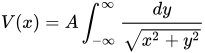
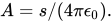
Since the charged line has 1-dimensional "spherical symmetry" (which in 1-dimension is just mirror symmetry), we can rewrite the integral to exploit the spherical symmetry: $\int _{-\infty }^{\infty }{\frac {dy}{\sqrt {x^{2}+y^{2}}}}=\int _{-\infty }^{\infty }{\frac {dt}{\sqrt {(x/x_{0})^{2}+t^{2}}}}=\int _{0}^{\infty }{\frac {\mathrm {vol} (S^{1})dr}{\sqrt {(x/x_{0})^{2}+r^{2}}}}$ where we first removed the dependence on length by dividing with a unit-length $x_{0}$ , then converted the integral over $\mathbb {R} ^{1}$ into an integral over the 1-sphere $S^{1}$ , followed by an integral over all radii of the 1-sphere.

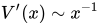
Now we generalize this into dimension $d$ . The volume of a d-sphere is ${\frac {2\pi ^{d/2}}{\Gamma (d/2)}}$ , where $\Gamma$ is the gamma function. Now the integral becomes ${\frac {2\pi ^{d/2}}{\Gamma (d/2)}}\int _{0}^{\infty }{\frac {r^{d-1}dr}{\sqrt {(x/x_{0})^{2}+r^{2}}}}$ When $d=1-\epsilon$ , the integral is dominated by its tail, that is, $\int _{0}^{\infty }{\frac {r^{d-1}dr}{\sqrt {(x/x_{0})^{2}+r^{2}}}}\sim \int _{c}^{\infty }r^{d-2}dr={\frac {1}{d-1}}c^{d-1}=\epsilon ^{-1}c^{-\epsilon },$ where $c=\Theta (x/x_{0})$ (in big Theta notation). Thus $V(x)\sim (x_{0}/x)^{\epsilon }/\epsilon$ , and so the electric field is $V'(x)\sim x^{-1}$ , as it should.

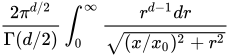
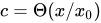
02Example

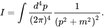
Suppose one wishes to dimensionally regularize a loop integral which is logarithmically divergent in four dimensions, like

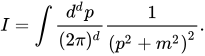
$I=\int {\frac {d^{4}p}{(2\pi )^{4}}}{\frac {1}{\left(p^{2}+m^{2}\right)^{2}}}.$

First, write the integral in a general non-integer number of dimensions $d=4-\varepsilon$ , where $\varepsilon$ will later be taken to be small, $I=\int {\frac {d^{d}p}{(2\pi )^{d}}}{\frac {1}{\left(p^{2}+m^{2}\right)^{2}}}.$ If the integrand only depends on $p^{2}$ , we can apply the formula $\int d^{d}p\,f(p^{2})={\frac {2\pi ^{d/2}}{\Gamma (d/2)}}\int _{0}^{\infty }dp\,p^{d-1}f(p^{2}).$ For integer dimensions like $d=3$ , this formula reduces to familiar integrals over thin shells like ${\textstyle \int _{0}^{\infty }dp\,4\pi p^{2}f(p^{2})$ . For non-integer dimensions, we define the value of the integral in this way by analytic continuation. This gives $I=\int _{0}^{\infty }{\frac {dp}{(2\pi )^{4-\varepsilon }}}{\frac {2\pi ^{(4-\varepsilon )/2}}{\Gamma \left({\frac {4-\varepsilon }{2}}\right)}}{\frac {p^{3-\varepsilon }}{\left(p^{2}+m^{2}\right)^{2}}}={\frac {2^{\varepsilon -4}\pi ^{{\frac {\varepsilon }{2}}-1}}{\sin \left({\frac {\pi \varepsilon }{2}}\right)\Gamma \left(1-{\frac {\varepsilon }{2}}\right)}}m^{-\varepsilon }={\frac {1}{8\pi ^{2}\varepsilon }}-{\frac {1}{16\pi ^{2}}}\left(\ln {\frac {m^{2}}{4\pi }}+\gamma \right)+{\mathcal {O}}(\varepsilon ).$ Note that the integral again diverges as $\varepsilon \rightarrow 0$ , but is finite for arbitrary small values $\varepsilon \neq 0$ .

Watch videos about Dimensional regularizationExplainers and documentaries on YouTube (opens in a new tab)

Sources and credits

This article is adapted from the Wikipedia article “Dimensional regularization”, written by its contributors and licensed under CC BY-SA 4.0. Fathomly has changed the layout, removed citation markers, navigation and maintenance notices, and adjusted punctuation. This adapted version is shared under the same license. For references, see the original article.

Fathomly is not affiliated with or endorsed by the Wikimedia Foundation. Spotted a problem? Tell us.