Digital delay line
Audio effect
A digital delay line (or simply delay line, also called delay filter) is a discrete element in a digital filter that allows a signal to be delayed by a number of samples. Delay lines are commonly used to delay audio signals feeding loudspeakers to compensate for the speed of sound in air, and to align video signals with accompanying audio, called audio-to-video synchronization. Delay lines may compensate for electronic processing latency so that multiple signals leave a device simultaneously despite having different pathways.
Digital delay lines are widely used building blocks in methods to simulate room acoustics, musical instruments and effects units. Digital waveguide synthesis shows how digital delay lines can be used as sound synthesis methods for various musical instruments such as string instruments and wind instruments.
If a delay line holds a non-integer value smaller than one, it results in a fractional delay line (also called interpolated delay line or fractional delay filter). A series of an integer delay line and a fractional delay filter is commonly used for modelling arbitrary delay filters in digital signal processing. The Dattorro scheme is an industry standard implementation of digital filters using fractional delay lines.
01Theory
The standard delay line with integer delay is derived from the Z-transform of a discrete-time signal 

![y[n]=x[n-M]](https://wikimedia.org/api/rest_v1/media/math/render/svg/40be9731d2f9971f62f4f5b6995068cc557545a6)
![{\xrightarrow[{}]{\mathcal {Z}}}](https://wikimedia.org/api/rest_v1/media/math/render/svg/180b260268ef119be0ea81daede2ca6c708dd0d1)
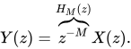
In this case, 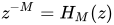
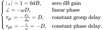
![{\begin{cases}|\centerdot |=1=0dB,&{\text{zero dB gain}}\\\measuredangle =-\omega M,&{\text{linear phase with }}\omega =2\pi fT_{s}{\text{ where }}T_{s}{\text{ is the sampling period in seconds }}[s].\end{cases}}](https://wikimedia.org/api/rest_v1/media/math/render/svg/3fbf6ae79953a07bbaada9ff38b6887211a55576)
The discrete-time domain filter for integer delay 
![h_{m}[n]={\begin{cases}{\text{1}},&{\text{for }}n=M\\0,&{\text{for }}n\neq M.\end{cases}}](https://wikimedia.org/api/rest_v1/media/math/render/svg/d2c4337d2e89786faf8772e961c3d018318d944f)
Working in the discrete-time domain with fractional delays is less trivial. In its most general theoretical form, a delay line with arbitrary fractional delay is defined as a standard delay line with delay 


 Domain
 | Def. 1 |
This is the 


02Filter design solutions
Naive solution
The conceptually easiest solution is obtained by sampling the continuous-time domain solution, which is trivial for any delay value. Given a continuous-time signal 

![{\xrightarrow[{}]{\mathcal {F}}}](https://wikimedia.org/api/rest_v1/media/math/render/svg/9e48e1acd34b29b9fc0c38a6fd28da43bc747c48)

In this case, 
The naive solution for the sampled filter ![h_{ideal}[n]](https://wikimedia.org/api/rest_v1/media/math/render/svg/5a1930205fc5eb87a56219a42b47d4e8043fcc7a)


![h_{ideal}[n]={\mathcal {F}}^{-1}[H_{ideal}(\omega )]={1 \over {2\pi }}\int \limits _{-\pi }^{+\pi }e^{j\omega D}e^{j\omega n}d\omega =sinc(n-D)={sin(\pi (n-D)) \over {\pi (n-D)}}](https://wikimedia.org/api/rest_v1/media/math/render/svg/6f90373718f1ae945a4d905fc4ad70684adbf9bd)
The continuous-time domain 
- when the delay is an integer number of samples
, the sampled shifted
- when the delay is a fractional number of samples
Truncated causal FIR solution
The conceptually easiest implementable solution is the causal truncation of the naive solution above.
![h_{\tau }[n]={\begin{cases}sinc(n-D)&{\text{for }}0\leq n\leq N\\0&{\text{otherwise}}\end{cases}}\;\;\;\;\;{\text{where}}\;\;\;\;\;{N-1 \over {2}}<D<{N+1 \over {2}}\;\;\;\;\;{\text{and}}\;\;\;\;\;N\;{\text{is the order of the filter.}}](https://wikimedia.org/api/rest_v1/media/math/render/svg/925b9b1670137a5c7046c5db0a8a7a4aefcb7c5c)
Truncating the impulse response might however cause instability, which can be mitigated in a few ways:
- Windowing the truncated impulse response, therefore smoothing it. Note that in this case we have to add a further shift
in order to align the window and the
- General Least Square (GLS) Method: iteratively adjusts the frequency response by windowing a Least Square Integral Error design, which minimises the square integral error between ideal and truncated frequency responses of the filter, defined as:
![h_{\tau }[n]={\begin{cases}w(n-D)sinc(n-D)&{\text{for }}L\leq n\leq L+N\\0&{\text{otherwise}}\end{cases}}\;\;\;\;\;{\text{where}}\;\;\;\;\;L={\begin{cases}round(D)-{N \over {2}}&{\text{for even }}N\\\lfloor D\rfloor -{N-1 \over {2}}&{\text{for odd }}N\end{cases}}](https://wikimedia.org/api/rest_v1/media/math/render/svg/21426c2e39afd8536796e94432b2a17e0af4765e)

- Lagrange Interpolator (Maximally Flat Fractional Delay Filter): adds "flatness" constraints to the first N derivatives of the Least Square Integral Error. This method is of particular interest because it has a closed form solution:
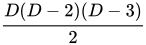
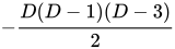
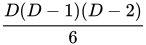
![h_{D}[n]=\prod _{k=0,\;k\neq n}^{N}{D-k \over {n-k}}\;\;\;\;\;{\text{where}}\;\;\;\;\;0\leq n\leq N](https://wikimedia.org/api/rest_v1/media/math/render/svg/6bf446da4e273efa8d0165ff30f4dbfb361000a5)
What follows is an expansion of the formula above displaying the resulting filters of order up to 
| Lagrange Interpolator Formula Expansion | ||||
|---|---|---|---|---|
![h_{\tau }[0]](https://wikimedia.org/api/rest_v1/media/math/render/svg/4bc4d76e82cde4b4dd5447b32774098e28f21b05) |
![h_{\tau }[1]](https://wikimedia.org/api/rest_v1/media/math/render/svg/131a2706c413350fd0a5444f8d531153434e77e2) |
![h_{\tau }[2]](https://wikimedia.org/api/rest_v1/media/math/render/svg/f38aa2571f36d7cfef3793075ca97486aead41d1) |
![h_{\tau }[3]](https://wikimedia.org/api/rest_v1/media/math/render/svg/06ce2107ddfbd2394aa3ffc5404fba5e2cf7a0e3) | |
| N = 1 |  |
|
- | - |
| N = 2 | 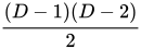 |
 |
 |
- |
| N = 3 | 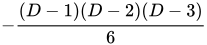 |
 |
 |
 |
All-pass IIR phase-approximated solution
Another approach is designing an IIR filter of order 

The reciprocally placed zeros and poles of 


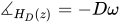
The main solutions are:
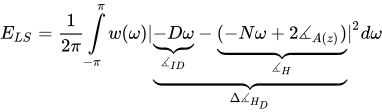
- Iterative minimization of Least Square Phase Error, which is defined as:
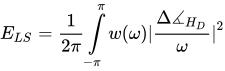
- Iterative minimization of Least Square Phase Delay Error, which is defined as:
- Thiran All-Pole Low-Pass Filter with Maximally Flat Group Delay. This yields a closed solution for finding the coefficients
:

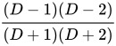
What follows is an expansion of the formula above displaying the resulting coefficients of order up to
| Thiran All-Pole Low-Pass Filter Coefficients Formula Expansion | ||||
|---|---|---|---|---|
 |
 |
 |
 | |
| N = 1 | 1 |  |
- | - |
| N = 2 | 1 |  |
 |
- |
| N = 3 | 1 |  |
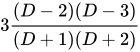 |
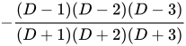 |

03Commercial history
Digital delay lines were first used to compensate for the speed of sound in air in 1973 to provide appropriate delay times for the distant speaker towers at the Summer Jam at Watkins Glen rock festival in New York, with 600,000 people in the audience. New York City-based company Eventide Clock Works provided digital delay devices each capable of 200 milliseconds of delay. Four speaker towers were placed 200 feet (60 m) from the stage, their signal delayed 175 ms to compensate for the speed of sound between the main stage speakers and the delay towers. Six more speaker towers were placed 400 feet from the stage, requiring 350 ms of delay, and a further six towers were placed 600 feet away from the stage, fed with 525 ms of delay. Each Eventide DDL 1745 module contained one hundred 1000-bit shift register chips and a bespoke digital-to-analog converter, and cost $3,800 (equivalent to $29,248 in 2025).

Sources and credits
This article is adapted from the Wikipedia article “Digital delay line”, written by its contributors and licensed under CC BY-SA 4.0. Fathomly has changed the layout, removed citation markers, navigation and maintenance notices, and adjusted punctuation. This adapted version is shared under the same license. For references, see the original article.
Images, from Wikimedia Commons:
- M-Sample Delay Line.png by Julius Smith, CC BY-SA 2.5
- Sampling of continuous-time domain sinc function at various fractional delay values.gif by Magiwanders, CC BY-SA 4.0
- Block Diagram for the Explicit Formula for Lagrange Interpolation Coefficients.png by Julius Smith, CC BY-SA 2.5
- DDL 1745-rack.jpg by Nalzatron, CC BY-SA 4.0
Fathomly is not affiliated with or endorsed by the Wikimedia Foundation. Spotted a problem? Tell us.
