Delta set
Abstraction useful in the construction and triangulation of topological spaces
In mathematics, a Δ-set, often called a Δ-complex or a semi-simplicial set, is a combinatorial object that is useful in the construction and triangulation of topological spaces, and also in the computation of related algebraic invariants of such spaces. A Δ-set is somewhat more general than a simplicial complex, yet not quite as sophisticated as a simplicial set. Simplicial sets have additional structure, so that every simplicial set is also a semi-simplicial set.
As an example, suppose we want to triangulate the 1-dimensional circle 
01Definition and related data
Formally, a Δ-set is a sequence of sets 

for each 


whenever 

This definition generalizes the notion of a simplicial complex, where the 


Given Δ-sets S and T, a map of Δ-sets is a collection of set-maps

such that

whenever both sides of the equation are defined.
With this notion, we can define the category of Δ-sets, whose objects are Δ-sets and whose morphisms are maps of Δ-sets.
Each Δ-set has a corresponding geometric realization, associating a geometrically defined space (a standard n-simplex) with each abstract simplex in Δ-set, and then "gluing" the spaces together using inclusion relations between the spaces to define an equivalence relation:
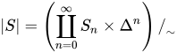
where we declare 

Here, 

is the inclusion of the i-th face. The geometric realization is a topological space with the quotient topology.
The geometric realization of a Δ-set S has a natural filtration

where
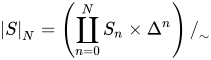
is a "restricted" geometric realization.

02Related functors
The geometric realization of a Δ-set described above defines a covariant functor from the category of Δ-sets to the category of topological spaces. Geometric realization takes a Δ-set to a topological space, and carries maps of Δ-sets to induced continuous maps between geometric realizations.
If S is a Δ-set, there is an associated free abelian chain complex, denoted 

generated by the set

This defines a covariant functor from the category of Δ-sets to the category of chain complexes of abelian groups. A Δ-set is carried to the chain complex just described, and a map of Δ-sets is carried to a map of chain complexes, which is defined by extending the map of Δ-sets in the standard way using the universal property of free abelian groups.
Given any topological space X, one can construct a Δ-set 

Define

to be the collection of all singular n-simplices in X, and define

by
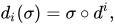
where again 

03Examples
This example illustrates the constructions described above. We can create a Δ-set S whose geometric realization is the unit circle

with 



It is simple to check that this is a Δ-set, and that 

where

In fact, 


All other homology groups are clearly trivial.
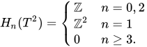
The following example is from section 2.1 of Hatcher's Algebraic Topology. Consider the Δ-set structure given to the torus in the figure, which has one vertex, three edges, and two 2-simplices.
The boundary map 






Since there are no 3-simplices, 



So 


Thus,
It is worth highlighting that the minimum number of simplices needed to endow 
This is a non-example. Consider a line segment. This is a 1-dimensional Δ-set and a 1-dimensional simplicial set. However, if we view the line segment as a 2-dimensional simplicial set, in which the 2-simplex is viewed as degenerate, then the line segment is not a Δ-set, as we do not allow for such degeneracies.
04Relation with simplical sets
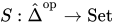
We now inspect the relation between Δ-sets and simplicial sets. Consider the simplex category 
![[n]:=\{0,1,\cdots ,n\}](https://wikimedia.org/api/rest_v1/media/math/render/svg/94d11e852fa68df4d24440a11270c8b8183b8258)


![\delta ^{i}:[n]\to [n+1]](https://wikimedia.org/api/rest_v1/media/math/render/svg/e82b9125874f5494e81c004608e7d8f83b24981d)
![i\in [n+1]](https://wikimedia.org/api/rest_v1/media/math/render/svg/5fd00828a795716f74083cfb7b5a0119f9bbe036)
![S([n])](https://wikimedia.org/api/rest_v1/media/math/render/svg/1f0d9d35b9eebcaaaf5b3339cfaefeecb49fbc77)





whenever 


From this perspective, it is now easy to see that every simplicial set is a Δ-set. Indeed, notice there is an inclusion 


05Pros and cons
One advantage of using Δ-sets in this way is that the resulting chain complex is generally much simpler than the singular chain complex. For reasonably simple spaces, all of the groups will be finitely generated, whereas the singular chain groups are, in general, not even countably generated.
One drawback of this method is that one must prove that the geometric realization of the Δ-set is actually homeomorphic to the topological space in question. This can become a computational challenge as the Δ-set increases in complexity.
Sources and credits
This article is adapted from the Wikipedia article “Delta set”, written by its contributors and licensed under CC BY-SA 4.0. Fathomly has changed the layout, removed citation markers, navigation and maintenance notices, and adjusted punctuation. This adapted version is shared under the same license. For references, see the original article.
Images, from Wikimedia Commons:
- Circle structures.svg by Homo morphisms, CC0
- Delta maps.svg by Homo morphisms, CC0
- Delta structures.pdf by Homo morphisms, CC0
Fathomly is not affiliated with or endorsed by the Wikimedia Foundation. Spotted a problem? Tell us.
