Delta method
Method in statistics
In statistics, the delta method is a method of deriving the asymptotic distribution of a random variable. It is applicable when the random variable being considered can be defined as a differentiable function of a random variable which is asymptotically Gaussian. More generally, the delta method applies to Hadamard directionally differentiable functionals of stochastic processes that converge to a limiting process.
01History
The delta method was derived from propagation of error, and the idea behind was known in the early 20th century. Its statistical application can be traced as far back as 1928 by T. L. Kelley. A formal description of the method was presented by J. L. Doob in 1935. Robert Dorfman also described a version of it in 1938.
02Univariate delta method
While the delta method generalizes easily to a multivariate setting, careful motivation of the technique is more easily demonstrated in univariate terms. Roughly, if there is a sequence of random variables Xn satisfying
![{{\sqrt {n}}[X_{n}-\theta ]\,\xrightarrow {D} \,{\mathcal {N}}(0,\sigma ^{2})},](https://wikimedia.org/api/rest_v1/media/math/render/svg/d0c0cc5e1bb093d98be669c7ee437eea66d30816)
where θ and σ2 are finite valued constants and 
![{{\sqrt {n}}[g(X_{n})-g(\theta )]\,\xrightarrow {D} \,{\mathcal {N}}(0,\sigma ^{2}\cdot [g'(\theta )]^{2})}](https://wikimedia.org/api/rest_v1/media/math/render/svg/e1c9662a6c08b9088cbbd6bd091b9c46033c07a2)
for any function g satisfying the property that its first derivative, evaluated at 

The intuition of the delta method is that any such g function, in a "small enough" range of the function, can be approximated via a first order Taylor polynomial, i.e., a linear function. If the random variable is roughly normal then a linear transformation of it is also normal. A small range can be ensured when approximating the function around the concentrating point of the sequence of random variables, so long as the variance is "small enough". When g is applied to a random variable such as the mean, the delta method would tend to work better as the sample size increases, since it would help reduce the variance, and thus the Taylor approximation would be applied to a smaller range of the function g at the point of interest.
Proof in the univariate case
Demonstration of this result is straightforward under the assumption that 


where 


where 

Rearranging the terms and multiplying by 
![{\sqrt {n}}[g(X_{n})-g(\theta )]=g'({\tilde {\theta }}_{n}){\sqrt {n}}[X_{n}-\theta ].](https://wikimedia.org/api/rest_v1/media/math/render/svg/fc218f4265097fcd5998be477476c36f0f43ba65)
Since
![{{\sqrt {n}}[X_{n}-\theta ]\xrightarrow {D} {\mathcal {N}}(0,\sigma ^{2})}](https://wikimedia.org/api/rest_v1/media/math/render/svg/9c66f8196a977e31de2cdc705d2dfd7924d58763)
by assumption, it follows from Slutsky's theorem that
![{{\sqrt {n}}[g(X_{n})-g(\theta )]\xrightarrow {D} {\mathcal {N}}(0,\sigma ^{2}[g'(\theta )]^{2})}.](https://wikimedia.org/api/rest_v1/media/math/render/svg/411bbe64fc07d9b513ed6f0219381bed0b8bd470)
This concludes the proof.
Proof with an explicit order of approximation
Alternatively, one can add one more step at the end, to obtain the order of approximation:
![{\begin{aligned}{\sqrt {n}}[g(X_{n})-g(\theta )]&=g'({\tilde {\theta }}_{n}){\sqrt {n}}[X_{n}-\theta ]\\[5pt]&={\sqrt {n}}[X_{n}-\theta ]\left[g'({\tilde {\theta }}_{n})+g'(\theta )-g'(\theta )\right]\\[5pt]&={\sqrt {n}}[X_{n}-\theta ]\left[g'(\theta )\right]+{\sqrt {n}}[X_{n}-\theta ]\left[g'({\tilde {\theta }}_{n})-g'(\theta )\right]\\[5pt]&={\sqrt {n}}[X_{n}-\theta ]\left[g'(\theta )\right]+O_{p}(1)\cdot o_{p}(1)\\[5pt]&={\sqrt {n}}[X_{n}-\theta ]\left[g'(\theta )\right]+o_{p}(1).\end{aligned}}](https://wikimedia.org/api/rest_v1/media/math/render/svg/5fb18715d74e5a646eb336c86fd9e635e9506ece)
This demonstrates that the error in the approximation converges to 0 in probability.
03Multivariate delta method
By definition, a consistent estimator B converges in probability to its true value β, and often a central limit theorem can be applied to obtain asymptotic normality:

where n is the number of observations and Σ is a (symmetric positive semi-definite) covariance matrix. Suppose we want to estimate the variance of a scalar-valued function h of the estimator B. Keeping only the first two terms of the Taylor series, and using vector notation for the gradient, we can estimate h(B) as

which implies the variance of h(B) is approximately
![{\begin{aligned}\operatorname {Var} \left(h(B)\right)&\approx \operatorname {Var} \left(h(\beta )+\nabla h(\beta )^{T}\cdot (B-\beta )\right)\\[5pt]&=\operatorname {Var} \left(h(\beta )+\nabla h(\beta )^{T}\cdot B-\nabla h(\beta )^{T}\cdot \beta \right)\\[5pt]&=\operatorname {Var} \left(\nabla h(\beta )^{T}\cdot B\right)\\[5pt]&=\nabla h(\beta )^{T}\cdot \operatorname {Cov} (B)\cdot \nabla h(\beta )\\[5pt]&=\nabla h(\beta )^{T}\cdot {\frac {\Sigma }{n}}\cdot \nabla h(\beta )\end{aligned}}](https://wikimedia.org/api/rest_v1/media/math/render/svg/1a00c9975a111a65f01d3e63cdfbe131c5328b61)
One can use the mean value theorem (for real-valued functions of many variables) to see that this does not rely on taking first order approximation.
The delta method therefore implies that

or in univariate terms,

04Example: the binomial proportion
Suppose Xn is binomial with parameters ![p\in (0,1]](https://wikimedia.org/api/rest_v1/media/math/render/svg/fc11ca62a414431ebe4c2411bc5931fa9dfbf66e)
![{{\sqrt {n}}\left[{\frac {X_{n}}{n}}-p\right]\,\xrightarrow {D} \,N(0,p(1-p))},](https://wikimedia.org/api/rest_v1/media/math/render/svg/f68936fde52a2d07cb6394ee23727f4e96300bd9)
we can apply the Delta method with g(θ) = log(θ) to see
![{{\sqrt {n}}\left[\log \left({\frac {X_{n}}{n}}\right)-\log(p)\right]\,\xrightarrow {D} \,N(0,p(1-p)[1/p]^{2})}](https://wikimedia.org/api/rest_v1/media/math/render/svg/500d2fd163eccb08acb6cb29e70516c27984d328)
Hence, even though for any finite n, the variance of 

Note that since p>0, 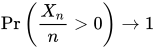

Moreover, if 


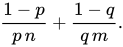
This is useful to construct a hypothesis test or to make a confidence interval for the relative risk.
05Alternative form
The delta method is often used in a form that is essentially identical to that above, but without the assumption that Xn or B is asymptotically normal. Often the only context is that the variance is "small". The results then just give approximations to the means and covariances of the transformed quantities. For example, the formulae presented in Klein (1953, p. 258) are:

where hr is the rth element of h(B) and Bi is the ith element of B.
06Second-order delta method
When g′(θ) = 0 the delta method cannot be applied. However, if g′′(θ) exists and is not zero, the second-order delta method can be applied. By the Taylor expansion, ![n[g(X_{n})-g(\theta )]={\frac {1}{2}}n[X_{n}-\theta ]^{2}\left[g''(\theta )\right]+o_{p}(1)](https://wikimedia.org/api/rest_v1/media/math/render/svg/ff5c652906bfd31ee2944c1b8430807dd0093acc)


Note that when using the second-order method, the expectation of g(Xn) is no longer simply g(θ), but also has a correction term that depends on the curvature: ![E[g(X_{n})]\approx g(\theta )+{\frac {1}{2}}g''(\theta )\sigma ^{2}](https://wikimedia.org/api/rest_v1/media/math/render/svg/e86500d474878c7db688f4329cffc918ec06044b)
The second-order delta method is also useful in conducting a more accurate approximation of ![{\sqrt {n}}[g(X_{n})-g(\theta )]={\sqrt {n}}[X_{n}-\theta ]g'(\theta )+{\frac {1}{2}}{\frac {n[X_{n}-\theta ]^{2}}{\sqrt {n}}}g''(\theta )+o_{p}(1)](https://wikimedia.org/api/rest_v1/media/math/render/svg/4fea000ed90e5a50e10d68a78ba790f44a41d130)
07Nonparametric delta method
A version of the delta method exists in nonparametric statistics. Let 


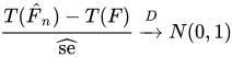
where 
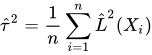
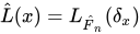


where 

Examples
In the following examples, 


Mean
For the mean functional

contamination of 

Therefore, the influence function is

Since 

Consequently,

and the standard error obtained from the general formula above is

Correlation coefficient
Let 
![T(F)=\rho ={\frac {\operatorname {E} [XY]-\operatorname {E} [X]\operatorname {E} [Y]}{\sqrt {\operatorname {Var} (X)\operatorname {Var} (Y)}}}.](https://wikimedia.org/api/rest_v1/media/math/render/svg/a2e72b6f091383b6c2520d4ca3a73f5c1452c03f)
Writing

the influence function of the correlation functional is

Let

and let 

Thus, the variance factor in the general standard-error formula may be estimated by

Quantile
Let

be the quantile of order 


If 


It follows that

At the population level,
![\operatorname {E} _{F}[L_{F}^{2}(X)]={\frac {p(1-p)}{f(q_{p})^{2}}},](https://wikimedia.org/api/rest_v1/media/math/render/svg/06edb4ab285ef00b7e471342e9eb882e621ec18c)
so the asymptotic variance of the sample quantile is

Sources and credits
This article is adapted from the Wikipedia article “Delta method”, written by its contributors and licensed under CC BY-SA 4.0. Fathomly has changed the layout, removed citation markers, navigation and maintenance notices, and adjusted punctuation. This adapted version is shared under the same license. For references, see the original article.
Fathomly is not affiliated with or endorsed by the Wikimedia Foundation. Spotted a problem? Tell us.