Encyclopedia

Debye function

Mathematical function

Wikipedia contributorsAdapted for Fathomly · View authors

2 min read
Source updated June 23, 2024

In mathematics, the family of Debye functions is defined by $D_{n}(x)={\frac {n}{x^{n}}}\int _{0}^{x}{\frac {t^{n}}{e^{t}-1}}\,dt.$

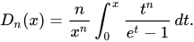
The functions are named in honor of Peter Debye, who came across this function (with n = 3) in 1912 when he analytically computed the heat capacity of what is now called the Debye model.

01Mathematical properties

Relation to other functions

The Debye functions are closely related to the polylogarithm.

Series expansion

They have the series expansion $D_{n}(x)=1-{\frac {n}{2(n+1)}}x+n\sum _{k=1}^{\infty }{\frac {B_{2k}}{(2k+n)(2k)!}}x^{2k},\quad |x|<2\pi ,\ n\geq 1,$ where $B_{n}$ is the n-th Bernoulli number.

Limiting values

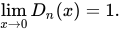
$\lim _{x\to 0}D_{n}(x)=1.$ If $\Gamma$ is the gamma function and $\zeta$ is the Riemann zeta function, then, for $x\gg 0$ , $D_{n}(x)={\frac {n}{x^{n}}}\int _{0}^{x}{\frac {t^{n}\,dt}{e^{t}-1}}\sim {\frac {n}{x^{n}}}\Gamma (n+1)\zeta (n+1),\qquad \operatorname {Re} n>0,$

Derivative

The derivative obeys the relation $xD_{n}^{\prime }(x)=n\left(B(x)-D_{n}(x)\right),$ where $B(x)=x/(e^{x}-1)$ is the Bernoulli function.

02Applications in solid-state physics

The Debye model

The Debye model has a density of vibrational states $g_{\text{D}}(\omega )={\frac {9\omega ^{2}}{\omega _{\text{D}}^{3}}}\,,\qquad 0\leq \omega \leq \omega _{\text{D}}$ with the Debye frequency ω_D.

Internal energy and heat capacity

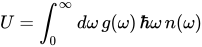
Inserting g into the internal energy $U=\int _{0}^{\infty }d\omega \,g(\omega )\,\hbar \omega \,n(\omega )$ with the Bose-Einstein distribution $n(\omega )={\frac {1}{\exp(\hbar \omega /k_{\text{B}}T)-1}}.$ one obtains $U=3k_{\text{B}}T\,D_{3}(\hbar \omega _{\text{D}}/k_{\text{B}}T).$ The heat capacity is the derivative thereof.

Mean squared displacement

The intensity of X-ray diffraction or neutron diffraction at wavenumber q is given by the Debye-Waller factor or the Lamb-Mössbauer factor. For isotropic systems it takes the form $\exp(-2W(q))=\exp \left(-q^{2}\langle u_{x}^{2}\rangle \right).$ In this expression, the mean squared displacement refers to just once Cartesian component u_x of the vector u that describes the displacement of atoms from their equilibrium positions. Assuming harmonicity and developing into normal modes, one obtains $2W(q)={\frac {\hbar ^{2}q^{2}}{6Mk_{\text{B}}T}}\int _{0}^{\infty }d\omega {\frac {k_{\text{B}}T}{\hbar \omega }}g(\omega )\coth {\frac {\hbar \omega }{2k_{\text{B}}T}}={\frac {\hbar ^{2}q^{2}}{6Mk_{\text{B}}T}}\int _{0}^{\infty }d\omega {\frac {k_{\text{B}}T}{\hbar \omega }}g(\omega )\left[{\frac {2}{\exp(\hbar \omega /k_{\text{B}}T)-1}}+1\right].$ Inserting the density of states from the Debye model, one obtains $2W(q)={\frac {3}{2}}{\frac {\hbar ^{2}q^{2}}{M\hbar \omega _{\text{D}}}}\left[2\left({\frac {k_{\text{B}}T}{\hbar \omega _{\text{D}}}}\right)D_{1}{\left({\frac {\hbar \omega _{\text{D}}}{k_{\text{B}}T}}\right)}+{\frac {1}{2}}\right].$ From the above power series expansion of $D_{1}$ follows that the mean square displacement at high temperatures is linear in temperature $2W(q)={\frac {3k_{\text{B}}Tq^{2}}{M\omega _{\text{D}}^{2}}}.$ The absence of $\hbar$ indicates that this is a classical result. Because $D_{1}(x)$ goes to zero for $x\to \infty$ it follows that for $T=0$ $2W(q)={\frac {3}{4}}{\frac {\hbar ^{2}q^{2}}{M\hbar \omega _{\text{D}}}}$ (zero-point motion).

03Implementations

Ng, E. W.; Devine, C. J. (1970). "On the computation of Debye functions of integer orders". Math. Comp. 24 (110): 405, 407. doi:10.1090/S0025-5718-1970-0272160-6. MR 0272160.
Engeln, I.; Wobig, D. (1983). "Computation of the generalized Debye functions delta(x,y) and D(x,y)". Colloid & Polymer Science. 261: 736, 743. doi:10.1007/BF01410947. S2CID 98476561.
MacLeod, Allan J. (1996). "Algorithm 757: MISCFUN, a software package to compute uncommon special functions". ACM Trans. Math. Software. 22 (3): 288, 301. doi:10.1145/232826.232846. S2CID 37814348. Fortran 77 code
Fortran 90 version
Maximon, Leonard C. (2003). "The dilogarithm function for complex argument". Proc. R. Soc. A. 459 (2039): 2807, 2819. Bibcode:2003RSPSA.459.2807M. doi:10.1098/rspa.2003.1156. S2CID 122271244.
Guseinov, I. I.; Mamedov, B. A. (2007). "Calculation of Integer and noninteger n-Dimensional Debye Functions using Binomial Coefficients and Incomplete Gamma Functions". Int. J. Thermophys. 28 (4): 1420, 1426. Bibcode:2007IJT....28.1420G. doi:10.1007/s10765-007-0256-1. S2CID 120284032.
C version of the GNU Scientific Library

Watch videos about Debye functionExplainers and documentaries on YouTube (opens in a new tab)

Sources and credits

This article is adapted from the Wikipedia article “Debye function”, written by its contributors and licensed under CC BY-SA 4.0. Fathomly has changed the layout, removed citation markers, navigation and maintenance notices, and adjusted punctuation. This adapted version is shared under the same license. For references, see the original article.

Fathomly is not affiliated with or endorsed by the Wikimedia Foundation. Spotted a problem? Tell us.