Dawson function
Mathematical function

In mathematics, the Dawson function or Dawson integral (named after H. G. Dawson) is the one-sided Fourier-Laplace sine transform of the Gaussian function.
01Definition
The Dawson function is defined as either:
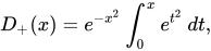


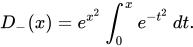
The Dawson function is the one-sided Fourier-Laplace sine transform of the Gaussian function,

It is closely related to the error function erf, as

where erfi is the imaginary error function, erfi(x) = −i erf(ix).
Similarly,
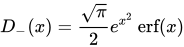
In terms of either erfi or the Faddeeva function 
![F(z)={{\sqrt {\pi }} \over 2}e^{-z^{2}}\operatorname {erfi} (z)={\frac {i{\sqrt {\pi }}}{2}}\left[e^{-z^{2}}-w(z)\right],](https://wikimedia.org/api/rest_v1/media/math/render/svg/5e4707739a168d777d1f57cd944ce6872c9fd4c1)
![D_{+}(x)=F(x)={\frac {\sqrt {\pi }}{2}}\operatorname {Im} [w(x)]](https://wikimedia.org/api/rest_v1/media/math/render/svg/5263fe3be9abf87a3afe139c5b8c41e809fce58f)
![D_{-}(x)=iF(-ix)=-{\frac {\sqrt {\pi }}{2}}\left[e^{x^{2}}-w(-ix)\right]](https://wikimedia.org/api/rest_v1/media/math/render/svg/bc7a357d8241fa43ece147f1a877841d56529118)

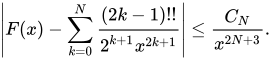
For 



More precisely

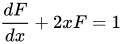


Inflection points follow for
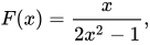


02Relation to Hilbert transform of Gaussian
The Hilbert transform of the Gaussian is defined as
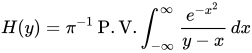
P.V. denotes the Cauchy principal value, and we restrict ourselves to real 



With 

![\pi H(y)=\operatorname {Im} \int _{0}^{\infty }dk\,\exp[-k^{2}/4+iky]\int _{-\infty }^{\infty }dx\,\exp[-(x+ik/2)^{2}].](https://wikimedia.org/api/rest_v1/media/math/render/svg/12890dc8ea10fe76bb211d705dbc25275718737d)
We can shift the integral over 
![\pi ^{1/2}H(y)=\operatorname {Im} \int _{0}^{\infty }dk\,\exp[-k^{2}/4+iky].](https://wikimedia.org/api/rest_v1/media/math/render/svg/1616202e4a1cd74e86616183e3e4a845aec1cc02)
We complete the square with respect to 
![\pi ^{1/2}H(y)=e^{-y^{2}}\operatorname {Im} \int _{0}^{\infty }dk\,\exp[-(k/2-iy)^{2}].](https://wikimedia.org/api/rest_v1/media/math/render/svg/28fb5c23b8ffaa8bf82e0b03e78cc572c0b94305)
We change variables to 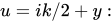

The integral can be performed as a contour integral around a rectangle in the complex plane. Taking the imaginary part of the result gives


The Hilbert transform of 
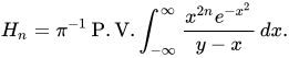
Introduce
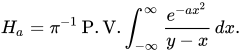
The 

We thus find
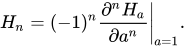
The derivatives are performed first, then the result evaluated at 










Sources and credits
This article is adapted from the Wikipedia article “Dawson function”, written by its contributors and licensed under CC BY-SA 4.0. Fathomly has changed the layout, removed citation markers, navigation and maintenance notices, and adjusted punctuation. This adapted version is shared under the same license. For references, see the original article.
Images, from Wikimedia Commons:
- Plot of the Dawson integral function F(z) in the complex plane from -2-2i to 2+2i with colors created with Mathematica 13.1 function ComplexPlot3D.svg by WalkingRadiance, CC BY-SA 4.0
- DawsonDp.svg by LSzilard, CC BY-SA 3.0
- DawsonDm.svg by LSzilard, CC BY-SA 3.0
Fathomly is not affiliated with or endorsed by the Wikimedia Foundation. Spotted a problem? Tell us.