Encyclopedia

Costas loop

Phase-locked loop-based demodulator circuit

Wikipedia contributorsAdapted for Fathomly · View authors

3 min read
Source updated November 26, 2025

A Costas loop is a phase-locked loop (PLL) based circuit which is used for carrier frequency recovery from suppressed-carrier modulation signals (e.g. double-sideband suppressed carrier signals) and phase modulation signals (e.g. BPSK, QPSK). It was invented by John P. Costas at General Electric in the 1950s. Its invention was described as having had "a profound effect on modern digital communications". The primary application of Costas loops is in wireless receivers. Its advantage over other PLL-based detectors is that at small deviations the Costas loop error voltage is 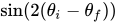$\sin(2(\theta _{i}-\theta _{f}))$ as compared to $\sin(\theta _{i}-\theta _{f})$ . This translates to double the sensitivity and also makes the Costas loop uniquely suited for tracking Doppler-shifted carriers, especially in OFDM and GPS receivers.

01Classical implementation

In the classical implementation of a Costas loop, a local voltage-controlled oscillator (VCO) provides quadrature outputs, one to each of two phase detectors, e.g., product detectors. The same phase of the input signal is also applied to both phase detectors, and the output of each phase detector is passed through a low-pass filter. The outputs of these low-pass filters are inputs to another phase detector, the output of which passes through a noise-reduction filter before being used to control the voltage-controlled oscillator. The coupled in-phase coherent detector and quadrature-phase coherent detector provide negative feedback to ensure the oscillator is synchronous with the carrier wave.

The overall loop response is controlled by the two individual low-pass filters that precede the third phase detector, while the third low-pass filter serves a trivial role in terms of gain and phase margin. The above figure of a Costas loop is drawn under the "locked" state, where the VCO frequency and the incoming carrier frequency have become the same due to the Costas loop process. The figure does not represent the "unlocked" state.

02Mathematical models

In the time domain

In the simplest case $m^{2}(t)=1$ . Therefore, $m^{2}(t)=1$ does not affect the input of the noise-reduction filter. The carrier and voltage-controlled oscillator (VCO) signals are periodic oscillations $f_{ref,vco}(\theta _{ref,vco}(t))$ with high-frequencies ${\dot {\theta }}_{ref,vco}(t)$ . The block $\bigotimes$ is an analog multiplier.

A linear filter can be described mathematically by a system of linear differential equations:

${\begin{array}{ll}{\dot {x}}=Ax+bu_{d}(t),&u_{LF}=c^{*}x.\end{array}}$

where $A$ is a constant matrix, $x(t)$ is a state vector of the filter, $b$ and $c$ are constant vectors.

The model of a VCO is usually assumed to be linear:

${\begin{array}{ll}{\dot {\theta }}_{vco}(t)=\omega _{vco}^{free}+K_{vco}u_{LF}(t),&t\in [0,T],\end{array}}$

where $\omega _{vco}^{free}$ is the free-running frequency of the VCO and $K_{vco}$ is the VCO gain factor. Similarly, it is possible to consider various nonlinear models of VCO.

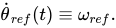
Suppose that the frequency of the master generator is constant ${\dot {\theta }}_{ref}(t)\equiv \omega _{ref}.$ Equation of VCO and equation of filter yield

${\begin{array}{ll}{\dot {x}}=Ax+bf_{ref}(\theta _{ref}(t))f_{vco}(\theta _{vco}(t)),&{\dot {\theta }}_{vco}=\omega _{vco}^{free}+K_{vco}c^{*}x.\end{array}}$

The system is non-autonomous and rather tricky for investigation.

In the phase-frequency domain

In the simplest case, when

${\begin{aligned}f_{ref}{\big (}\theta _{ref}(t){\big )}=\cos {\big (}\omega _{ref}t{\big )},\ f_{vco}{\big (}\theta _{vco}(t){\big )}&=\sin {\big (}\theta _{vco}(t){\big )}\\f_{ref}{\big (}\theta _{ref}(t){\big )}^{2}f_{vco}\left(\theta _{vco}(t)\right)f_{vco}\left(\theta _{vco}(t)-{\frac {\pi }{2}}\right)&=-{\frac {1}{8}}{\Big (}2\sin(2\theta _{vco}(t))+\sin(2\theta _{vco}(t)-2\omega _{ref}t)+\sin(2\theta _{vco}(t)+2\omega _{ref}t){\Big )}\end{aligned}}$

The standard engineering assumption is that the filter removes the upper sideband frequency from the input but leaves the lower sideband without change. Thus it is assumed that the VCO input is $\varphi (\theta _{ref}(t)-\theta _{vco}(t))={\frac {1}{8}}\sin(2\omega _{ref}t-2\theta _{vco}(t)).$ This makes a Costas loop equivalent to a phase-locked loop with phase detector characteristic $\varphi (\theta )$ corresponding to the particular waveforms $f_{ref}(\theta )$ and $f_{vco}(\theta )$ of the input and VCO signals. It can be proved that filter outputs in the time and phase-frequency domains are almost equal.

Thus it is possible to study the simpler autonomous system of differential equations

${\begin{aligned}{\dot {x}}&=Ax+b\varphi (\Delta \theta ),\\\Delta {\dot {\theta }}&=\omega _{vco}^{free}-\omega _{ref}+K_{vco}c^{*}x,\\\Delta \theta &=\theta _{vco}-\theta _{ref}.\end{aligned}}$ .

The Krylov-Bogoliubov averaging method allows one to prove that solutions of non-autonomous and autonomous equations are close under some assumptions. Thus, the Costas loop block diagram in the time domain can be asymptotically changed to the block diagram on the level of phase-frequency relations.

The transition to the analysis of an autonomous dynamical model of the Costas loop (in place of the non-autonomous one) allows one to overcome the difficulties related to modeling the Costas loop in the time domain, where one has to simultaneously observe a very fast time scale of the input signals and slow time scale of signal's phase. This idea makes it possible to calculate core performance characteristics - hold-in, pull-in, and lock-in ranges.

Equivalent phase-frequency domain model of Costas loop

03Frequency acquisition

The classical Costas loop will work towards making the phase difference between the carrier and the VCO become a small, ideally zero, value. The small phase difference implies that frequency lock has been achieved.

04QPSK Costas loop

The classical Costas loop can be adapted to QPSK modulation for higher data rates.

The input QPSK signal is as follows

$m_{1}(t)\cos \left(\omega _{\text{ref}}t\right)+m_{2}(t)\sin \left(\omega _{\text{ref}}t\right),m_{1}(t)=\pm 1,m_{2}(t)=\pm 1.$

Inputs of low-pass filters LPF1 and LPF2 are

${\begin{aligned}\varphi _{1}(t)&=\cos \left(\theta _{\text{vco}}\right)\left(m_{1}(t)\cos \left(\omega _{\text{ref}}t\right)+m_{2}(t)\sin \left(\omega _{\text{ref}}t\right)\right),\\\varphi _{2}(t)&=\sin \left(\theta _{\text{vco}}\right)\left(m_{1}(t)\cos \left(\omega _{\text{ref}}t\right)+m_{2}(t)\sin \left(\omega _{\text{ref}}t\right)\right).\end{aligned}}$

After synchronization, the outputs of LPF1 $Q(t)$ and LPF2 $I(t)$ are used to get demodulated data ( $m_{1}(t)$ and $m_{2}(t)$ ). To adjust the frequency of the VCO to the reference frequency, signals $Q(t)$ and $I(t)$ are limited and cross-multiplied:

$u_{d}(t)=I(t)\operatorname {sgn} (Q(t))-Q(t)\operatorname {sgn} (I(t)).$

Then the signal $u_{d}(t)$ is filtered by the loop filter and forms the tuning signal for the VCO $u_{\text{LF}}(t)$ , similar to BPSK Costas loop. Thus, QPSK Costas can be described by a system of ordinary differential equations:

${\begin{aligned}{\dot {x}}_{1}&=A_{\text{LPF}}x_{1}+b_{\text{LPF}}\varphi _{1}(t),\\{\dot {x}}_{2}&=A_{\text{LPF}}x_{2}+b_{\text{LPF}}\varphi _{2}(t),\\{\dot {x}}&=A_{\text{LF}}x+b_{\text{LF}}{\big (}c_{\text{LPF}}^{*}x_{1}\operatorname {sgn} (c_{\text{LPF}}^{*}x_{2})-c_{\text{LPF}}^{*}x_{2}\operatorname {sgn} (c_{\text{LPF}}^{*}x_{1}){\big )},\\{\dot {\theta }}_{\text{vco}}&=\omega _{\text{vco}}^{\text{free}}+K_{\text{VCO}}{\Big (}c_{\text{LF}}^{*}x+h_{\text{LF}}{\big (}c_{\text{LPF}}^{*}x_{1}\operatorname {sgn} (c_{\text{LPF}}^{*}x_{2})-c_{\text{LPF}}^{*}x_{2}\operatorname {sgn} (c_{\text{LPF}}^{*}x_{1}){\big )}{\Big )}.\\\end{aligned}}$

Here $A_{\text{LPF}},b_{\text{LPF}},c_{\text{LPF}}$ are parameters of LPF1 and LPF2 and $A_{\text{LF}},b_{\text{LF}},c_{\text{LF}},h_{\text{LF}}$ are parameters of the loop filter.

Watch videos about Costas loopExplainers and documentaries on YouTube (opens in a new tab)

Sources and credits

This article is adapted from the Wikipedia article “Costas loop”, written by its contributors and licensed under CC BY-SA 4.0. Fathomly has changed the layout, removed citation markers, navigation and maintenance notices, and adjusted punctuation. This adapted version is shared under the same license. For references, see the original article.

Images, from Wikimedia Commons:

Costas loop model.svg by Marat Yuldashev, CC BY-SA 4.0
Costas-non-equal-freq-high-res.png by Maratyv, CC BY-SA 4.0
Costas-phase-pll-ics-high-res.png by Maratyv, CC BY-SA 4.0
PLL trainsient process phase domain.svg by Renatyv, CC BY-SA 3.0
Costas loop before sync.png by Renatyv, CC BY-SA 4.0
Costas loop after sync.png by Renatyv, CC BY-SA 4.0
Costas loop signals before sycnhronization.svg by Renatyv, CC BY-SA 3.0
Costas loop trainsient process.svg by Renatyv, CC BY-SA 3.0

Fathomly is not affiliated with or endorsed by the Wikimedia Foundation. Spotted a problem? Tell us.