Encyclopedia

Correlogram

Chart of correlation statistics

Wikipedia contributorsAdapted for Fathomly · View authors

4 min read
Source updated July 13, 2026

In the analysis of data, a correlogram is a chart of correlation statistics. For example, in time series analysis, a plot of the sample autocorrelations $r_{h}$ versus $h\,$ (the time lags) is an autocorrelogram. If cross-correlation is plotted, the result is called a cross-correlogram.

The correlogram is a commonly used tool for checking randomness in a data set. If random, autocorrelations should be near zero for any and all time-lag separations. If non-random, then one or more of the autocorrelations will be significantly non-zero.

In addition, correlograms are used in the model identification stage for Box-Jenkins autoregressive moving average time series models. Autocorrelations should be near-zero for randomness; if the analyst does not check for randomness, then the validity of many of the statistical conclusions becomes suspect. The correlogram is an excellent way of checking for such randomness.

In multivariate analysis, correlation matrices shown as color-mapped images may also be called "correlograms" or "corrgrams".

01Applications

The correlogram can help provide answers to the following questions:

Are the data random?
Is an observation related to an adjacent observation?
Is an observation related to an observation twice-removed? (etc.)
Is the observed time series white noise?
Is the observed time series sinusoidal?
Is the observed time series autoregressive?
What is an appropriate model for the observed time series?
Is the model

$Y={\text{constant}}+{\text{error}}$

valid and sufficient?

Is the formula $s_{\bar {Y}}=s/{\sqrt {N}}$ valid?

02Importance

Randomness (along with fixed model, fixed variation, and fixed distribution) is one of the four assumptions that typically underlie all measurement processes. The randomness assumption is critically important for the following three reasons:

Most standard statistical tests depend on randomness. The validity of the test conclusions is directly linked to the validity of the randomness assumption.
Many commonly used statistical formulae depend on the randomness assumption, the most common formula being the formula for determining the standard error of the sample mean:

$s_{\bar {Y}}=s/{\sqrt {N}}$

where s is the standard deviation of the data. Although heavily used, the results from using this formula are of no value unless the randomness assumption holds.

For univariate data, the default model is

$Y={\text{constant}}+{\text{error}}$

If the data are not random, this model is incorrect and invalid, and the estimates for the parameters (such as the constant) become nonsensical and invalid.

03Estimation of autocorrelations

The autocorrelation coefficient at lag h is given by

$r_{h}=c_{h}/c_{0}\,$

where c_h is the autocovariance function

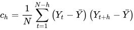
$c_{h}={\frac {1}{N}}\sum _{t=1}^{N-h}\left(Y_{t}-{\bar {Y}}\right)\left(Y_{t+h}-{\bar {Y}}\right)$

and c₀ is the variance function

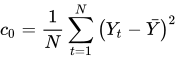
$c_{0}={\frac {1}{N}}\sum _{t=1}^{N}\left(Y_{t}-{\bar {Y}}\right)^{2}$

The resulting value of r_h will range between −1 and +1.

Alternate estimate

Some sources may use the following formula for the autocovariance function:

$c_{h}={\frac {1}{N-h}}\sum _{t=1}^{N-h}\left(Y_{t}-{\bar {Y}}\right)\left(Y_{t+h}-{\bar {Y}}\right)$

Although this definition has less bias, the (1/N) formulation has some desirable statistical properties and is the form most commonly used in the statistics literature. See pages 20 and 49-50 in Chatfield for details.

In contrast to the definition above, this definition allows us to compute $c_{h}$ in a slightly more intuitive way. Consider the sample $Y_{1},\dots ,Y_{N}$ , where $Y_{i}\in \mathbb {R} ^{n}$ for $i=1,\dots ,N$ . Then, let

$X={\begin{bmatrix}Y_{1}-{\bar {Y}}&\cdots &Y_{N}-{\bar {Y}}\end{bmatrix}}\in \mathbb {R} ^{n\times N}$

We then compute the Gram matrix $Q=X^{\top }X$ . Finally, $c_{h}$ is computed as the sample mean of the $h$ th diagonal of $Q$ . For example, the $0$ th diagonal (the main diagonal) of $Q$ has $N$ elements, and its sample mean corresponds to $c_{0}$ . The $1$ st diagonal (to the right of the main diagonal) of $Q$ has $N-1$ elements, and its sample mean corresponds to $c_{1}$ , and so on.

04Statistical inference with correlograms

In the same graph one can draw upper and lower bounds for autocorrelation with significance level $\alpha \,$ :

$B=\pm z_{1-\alpha /2}SE(r_{h})\,$ with $r_{h}\,$ as the estimated autocorrelation at lag $h\,$ .

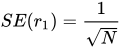
If the autocorrelation is higher (lower) than this upper (lower) bound, the null hypothesis that there is no autocorrelation at and beyond a given lag is rejected at a significance level of $\alpha \,$ . This test is an approximate one and assumes that the time-series is Gaussian.

In the above, z_1−α/2 is the quantile of the normal distribution; SE is the standard error, which can be computed by Bartlett's formula for MA(ℓ) processes:

$SE(r_{1})={\frac {1}{\sqrt {N}}}$

$SE(r_{h})={\sqrt {\frac {1+2\sum _{i=1}^{h-1}r_{i}^{2}}{N}}}$ for $h>1.\,$

In the example plotted, we can reject the null hypothesis that there is no autocorrelation between time-points which are separated by lags up to 4. For most longer periods one cannot reject the null hypothesis of no autocorrelation.

Note that there are two distinct formulas for generating the confidence bands:

1. If the correlogram is being used to test for randomness (i.e., there is no time dependence in the data), the following formula is recommended:

$\pm {\frac {z_{1-\alpha /2}}{\sqrt {N}}}$

where N is the sample size, z is the quantile function of the standard normal distribution and α is the significance level. In this case, the confidence bands have fixed width that depends on the sample size.

2. Correlograms are also used in the model identification stage for fitting ARIMA models. In this case, a moving average model is assumed for the data and the following confidence bands should be generated:

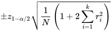
$\pm z_{1-\alpha /2}{\sqrt {{\frac {1}{N}}\left(1+2\sum _{i=1}^{k}r_{i}^{2}\right)}}$

where k is the lag. In this case, the confidence bands increase as the lag increases.

05Software

Correlograms are available in most general purpose statistical libraries.

Correlograms:

python pandas: pandas.plotting.autocorrelation_plot
R: functions acf and pacf

Corrgrams:

python seaborn: heatmap, pairplot
R: corrgram

Watch videos about CorrelogramExplainers and documentaries on YouTube (opens in a new tab)

Sources and credits

This article is adapted from the Wikipedia article “Correlogram”, written by its contributors and licensed under CC BY-SA 4.0. Fathomly has changed the layout, removed citation markers, navigation and maintenance notices, and adjusted punctuation. This adapted version is shared under the same license. For references, see the original article.

Images, from Wikimedia Commons:

Acf.svg by M. W. Toews, CC BY 4.0
Correlogram example.png by Dicklyon, CC BY-SA 4.0
Correlogram samples.png by Dicklyon, CC BY-SA 4.0

Fathomly is not affiliated with or endorsed by the Wikimedia Foundation. Spotted a problem? Tell us.