Encyclopedia

Complex normal distribution

Statistical distribution of complex random variables

Wikipedia contributorsAdapted for Fathomly · View authors

3 min read
Source updated September 6, 2026

In probability theory, the family of complex normal distributions, denoted ${\mathcal {CN}}$ or ${\mathcal {N}}_{\mathcal {C}}$ , characterizes complex random variables whose real and imaginary parts are jointly normal. The complex normal family has three parameters: location parameter μ, covariance matrix $\Gamma$ , and the relation matrix $C$ . The standard complex normal is the univariate distribution with $\mu =0$ , $\Gamma =1$ , and $C=0$ .

An important subclass of complex normal family is called the circularly-symmetric (central) complex normal and corresponds to the case of zero relation matrix and zero mean: $\mu =0$ and $C=0$ . This case is used extensively in signal processing, where it is sometimes referred to as just complex normal in the literature.

01Definitions

Complex standard normal random variable

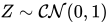
The standard complex normal random variable or standard complex Gaussian random variable is a complex random variable $Z$ whose real and imaginary parts are independent normally distributed random variables with mean zero and variance $1/2$ . Formally,

$Z\sim {\mathcal {CN}}(0,1)\quad \iff \quad \Re (Z)\perp \!\!\!\perp \Im (Z){\text{ and }}\Re (Z)\sim {\mathcal {N}}(0,1/2){\text{ and }}\Im (Z)\sim {\mathcal {N}}(0,1/2)$

Eq.1

where $\perp \!\!\!\perp$ denotes independence and $Z\sim {\mathcal {CN}}(0,1)$ denotes that $Z$ is a standard complex normal random variable.

Complex normal random variable

Suppose $X$ and $Y$ are real random variables such that $(X,Y)^{\mathrm {T} }$ is a 2-dimensional normal random vector. Then the complex random variable $Z=X+iY$ is called complex normal random variable or complex Gaussian random variable.

$Z{\text{ complex normal random variable}}\quad \iff \quad (\Re (Z),\Im (Z))^{\mathrm {T} }{\text{ real normal random vector}}$

Eq.2

Complex standard normal random vector

A n-dimensional complex random vector $\mathbf {Z} =(Z_{1},\ldots ,Z_{n})^{\mathrm {T} }$ is a complex standard normal random vector or complex standard Gaussian random vector if its components are independent and all of them are standard complex normal random variables as defined above. That $\mathbf {Z}$ is a standard complex normal random vector is denoted $\mathbf {Z} \sim {\mathcal {CN}}(0,{\boldsymbol {I}}_{n})$ .

$\mathbf {Z} \sim {\mathcal {CN}}(0,{\boldsymbol {I}}_{n})\quad \iff (Z_{1},\ldots ,Z_{n}){\text{ independent}}{\text{ and for }}1\leq i\leq n:Z_{i}\sim {\mathcal {CN}}(0,1)$

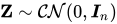
Eq.3

Complex normal random vector

If $\mathbf {X} =(X_{1},\ldots ,X_{n})^{\mathrm {T} }$ and $\mathbf {Y} =(Y_{1},\ldots ,Y_{n})^{\mathrm {T} }$ are random vectors in $\mathbb {R} ^{n}$ such that $[\mathbf {X} ,\mathbf {Y} ]$ is a normal random vector with $2n$ components. Then we say that the complex random vector

$\mathbf {Z} =\mathbf {X} +i\mathbf {Y} \,$

is a complex normal random vector or a complex Gaussian random vector.

$\mathbf {Z} {\text{ complex normal random vector}}\quad \iff \quad (\Re (\mathbf {Z} ^{\mathrm {T} }),\Im (\mathbf {Z} ^{\mathrm {T} }))^{\mathrm {T} }=(\Re (Z_{1}),\ldots ,\Re (Z_{n}),\Im (Z_{1}),\ldots ,\Im (Z_{n}))^{\mathrm {T} }{\text{ real normal random vector}}$

Eq.4

02Mean, covariance, and relation

The complex Gaussian distribution can be described with 3 parameters:

$\mu =\operatorname {E} [\mathbf {Z} ],\quad \Gamma =\operatorname {E} [(\mathbf {Z} -\mu )({\mathbf {Z} }-\mu )^{\mathrm {H} }],\quad C=\operatorname {E} [(\mathbf {Z} -\mu )(\mathbf {Z} -\mu )^{\mathrm {T} }],$

where $\mathbf {Z} ^{\mathrm {T} }$ denotes matrix transpose of $\mathbf {Z}$ , and $\mathbf {Z} ^{\mathrm {H} }$ denotes conjugate transpose.

Here the location parameter $\mu$ is a n-dimensional complex vector; the covariance matrix $\Gamma$ is Hermitian and non-negative definite; and, the relation matrix or pseudo-covariance matrix $C$ is symmetric. The complex normal random vector $\mathbf {Z}$ can now be denoted as $\mathbf {Z} \ \sim \ {\mathcal {CN}}(\mu ,\ \Gamma ,\ C).$ Moreover, matrices $\Gamma$ and $C$ are such that the matrix

$P={\overline {\Gamma }}-{C}^{\mathrm {H} }\Gamma ^{-1}C$

is also non-negative definite where ${\overline {\Gamma }}$ denotes the complex conjugate of $\Gamma$ .

03Relationships between covariance matrices

As for any complex random vector, the matrices $\Gamma$ and $C$ can be related to the covariance matrices of $\mathbf {X} =\Re (\mathbf {Z} )$ and $\mathbf {Y} =\Im (\mathbf {Z} )$ via expressions

${\begin{aligned}&V_{XX}\equiv \operatorname {E} [(\mathbf {X} -\mu _{X})(\mathbf {X} -\mu _{X})^{\mathrm {T} }]={\tfrac {1}{2}}\operatorname {Re} [\Gamma +C],\quad V_{XY}\equiv \operatorname {E} [(\mathbf {X} -\mu _{X})(\mathbf {Y} -\mu _{Y})^{\mathrm {T} }]={\tfrac {1}{2}}\operatorname {Im} [-\Gamma +C],\\&V_{YX}\equiv \operatorname {E} [(\mathbf {Y} -\mu _{Y})(\mathbf {X} -\mu _{X})^{\mathrm {T} }]={\tfrac {1}{2}}\operatorname {Im} [\Gamma +C],\quad \,V_{YY}\equiv \operatorname {E} [(\mathbf {Y} -\mu _{Y})(\mathbf {Y} -\mu _{Y})^{\mathrm {T} }]={\tfrac {1}{2}}\operatorname {Re} [\Gamma -C],\end{aligned}}$

and conversely

${\begin{aligned}&\Gamma =V_{XX}+V_{YY}+i(V_{YX}-V_{XY}),\\&C=V_{XX}-V_{YY}+i(V_{YX}+V_{XY}).\end{aligned}}$

04Density function

The probability density function for complex normal distribution can be computed as

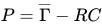
${\begin{aligned}f(z)&={\frac {1}{\pi ^{n}{\sqrt {\det(\Gamma )\det(P)}}}}\,\exp \!\left\{-{\frac {1}{2}}{\begin{bmatrix}z-\mu \\{\overline {z}}-{\overline {\mu }}\end{bmatrix}}^{\mathrm {H} }{\begin{bmatrix}\Gamma &C\\{\overline {C}}&{\overline {\Gamma }}\end{bmatrix}}^{\!\!-1}\!{\begin{bmatrix}z-\mu \\{\overline {z}}-{\overline {\mu }}\end{bmatrix}}\right\}\\[8pt]&={\tfrac {\sqrt {\det \left({\overline {P^{-1}}}-R^{\ast }P^{-1}R\right)\det(P^{-1})}}{\pi ^{n}}}\,e^{-(z-\mu )^{\ast }{\overline {P^{-1}}}(z-\mu )+\operatorname {Re} \left((z-\mu )^{\intercal }R^{\intercal }{\overline {P^{-1}}}(z-\mu )\right)},\end{aligned}}$

where $R=C^{\mathrm {H} }\Gamma ^{-1}$ and $P={\overline {\Gamma }}-RC$ .

05Characteristic function

The characteristic function of complex normal distribution is given by

$\varphi (w)=\exp \!{\big \{}i\operatorname {Re} ({\overline {w}}'\mu )-{\tfrac {1}{4}}{\big (}{\overline {w}}'\Gamma w+\operatorname {Re} ({\overline {w}}'C{\overline {w}}){\big )}{\big \}},$

where the argument $w$ is an n-dimensional complex vector.

06Properties

If $\mathbf {Z}$ is a complex normal n-vector, ${\boldsymbol {A}}$ an m×n matrix, and $b$ a constant m-vector, then the linear transform ${\boldsymbol {A}}\mathbf {Z} +b$ will be distributed also complex-normally:

$Z\ \sim \ {\mathcal {CN}}(\mu ,\,\Gamma ,\,C)\quad \Rightarrow \quad AZ+b\ \sim \ {\mathcal {CN}}(A\mu +b,\,A\Gamma A^{\mathrm {H} },\,ACA^{\mathrm {T} })$

If $\mathbf {Z}$ is a complex normal n-vector, then

$2{\Big [}(\mathbf {Z} -\mu )^{\mathrm {H} }{\overline {P^{-1}}}(\mathbf {Z} -\mu )-\operatorname {Re} {\big (}(\mathbf {Z} -\mu )^{\mathrm {T} }R^{\mathrm {T} }{\overline {P^{-1}}}(\mathbf {Z} -\mu ){\big )}{\Big ]}\ \sim \ \chi ^{2}(2n)$

Central limit theorem. If $Z_{1},\ldots ,Z_{T}$ are independent and identically distributed complex random variables, then

${\sqrt {T}}{\Big (}{\tfrac {1}{T}}\textstyle \sum _{t=1}^{T}Z_{t}-\operatorname {E} [Z_{t}]{\Big )}\ \xrightarrow {d} \ {\mathcal {CN}}(0,\,\Gamma ,\,C),$

where $\Gamma =\operatorname {E} [ZZ^{\mathrm {H} }]$ and $C=\operatorname {E} [ZZ^{\mathrm {T} }]$ .

The modulus of a complex normal random variable follows a Hoyt distribution.

07Circularly-symmetric central case

Definition

A complex random vector $\mathbf {Z}$ is called circularly symmetric if for every deterministic $\varphi \in [-\pi ,\pi )$ the distribution of $e^{\mathrm {i} \varphi }\mathbf {Z}$ equals the distribution of $\mathbf {Z}$ .

Central normal complex random vectors that are circularly symmetric are of particular interest because they are fully specified by the covariance matrix $\Gamma$ .

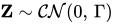
The circularly-symmetric (central) complex normal distribution corresponds to the case of zero mean and zero relation matrix, i.e. $\mu =0$ and $C=0$ . This is usually denoted

$\mathbf {Z} \sim {\mathcal {CN}}(0,\,\Gamma )$

Distribution of real and imaginary parts

If $\mathbf {Z} =\mathbf {X} +i\mathbf {Y}$ is circularly-symmetric (central) complex normal, then the vector $[\mathbf {X} ,\mathbf {Y} ]$ is multivariate normal with covariance structure

${\begin{pmatrix}\mathbf {X} \\\mathbf {Y} \end{pmatrix}}\ \sim \ {\mathcal {N}}{\Big (}{\begin{bmatrix}0\\0\end{bmatrix}},\ {\tfrac {1}{2}}{\begin{bmatrix}\operatorname {Re} \,\Gamma &-\operatorname {Im} \,\Gamma \\\operatorname {Im} \,\Gamma &\operatorname {Re} \,\Gamma \end{bmatrix}}{\Big )}$

where $\Gamma =\operatorname {E} [\mathbf {Z} \mathbf {Z} ^{\mathrm {H} }]$ .

Probability density function

For nonsingular covariance matrix $\Gamma$ , its distribution can also be simplified as

$f_{\mathbf {Z} }(\mathbf {z} )={\tfrac {1}{\pi ^{n}\det(\Gamma )}}\,e^{-(\mathbf {z} -\mathbf {\mu } )^{\mathrm {H} }\Gamma ^{-1}(\mathbf {z} -\mathbf {\mu } )}$ .

Therefore, if the non-zero mean $\mu$ and covariance matrix $\Gamma$ are unknown, a suitable log likelihood function for a single observation vector $z$ would be

$\ln(L(\mu ,\Gamma ))=-\ln(\det(\Gamma ))-{\overline {(z-\mu )}}'\Gamma ^{-1}(z-\mu )-n\ln(\pi ).$

The standard complex normal (defined in Eq.1) corresponds to the distribution of a scalar random variable with $\mu =0$ , $C=0$ and $\Gamma =1$ . Thus, the standard complex normal distribution has density

$f_{Z}(z)={\tfrac {1}{\pi }}e^{-{\overline {z}}z}={\tfrac {1}{\pi }}e^{-|z|^{2}}.$

Properties

The above expression demonstrates why the case $C=0$ , $\mu =0$ is called “circularly-symmetric”. The density function depends only on the magnitude of $z$ but not on its argument. As such, the magnitude $|z|$ of a standard complex normal random variable will have the Rayleigh distribution and the squared magnitude $|z|^{2}$ will have the exponential distribution, whereas the argument will be distributed uniformly on $[-\pi ,\pi ]$ .

If $\left\{\mathbf {Z} _{1},\ldots ,\mathbf {Z} _{k}\right\}$ are independent and identically distributed n-dimensional circular complex normal random vectors with $\mu =0$ , then the random squared norm

$Q=\sum _{j=1}^{k}\mathbf {Z} _{j}^{\mathrm {H} }\mathbf {Z} _{j}=\sum _{j=1}^{k}\|\mathbf {Z} _{j}\|^{2}$

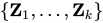
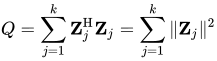
has the generalized chi-squared distribution and the random matrix

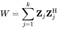
$W=\sum _{j=1}^{k}\mathbf {Z} _{j}\mathbf {Z} _{j}^{\mathrm {H} }$

has the complex Wishart distribution with $k$ degrees of freedom. This distribution can be described by density function

$f(w)={\frac {\det(\Gamma ^{-1})^{k}\det(w)^{k-n}}{\pi ^{n(n-1)/2}\prod _{j=1}^{k}(k-j)!}}\ e^{-\operatorname {tr} (\Gamma ^{-1}w)}$

where $k\geq n$ , and $w$ is a $n\times n$ nonnegative-definite matrix.

Watch videos about Complex normal distributionExplainers and documentaries on YouTube (opens in a new tab)

Sources and credits

This article is adapted from the Wikipedia article “Complex normal distribution”, written by its contributors and licensed under CC BY-SA 4.0. Fathomly has changed the layout, removed citation markers, navigation and maintenance notices, and adjusted punctuation. This adapted version is shared under the same license. For references, see the original article.

Fathomly is not affiliated with or endorsed by the Wikimedia Foundation. Spotted a problem? Tell us.