Bernoulli distribution
Probability distribution modeling a coin toss which need not be fair

In probability theory and statistics, the Bernoulli distribution, named after Swiss mathematician Jacob Bernoulli, is the discrete probability distribution of a random variable which takes the value 1 with probability 


The Bernoulli distribution is a special case of the binomial distribution where a single trial is conducted (so n would be 1 for such a binomial distribution). It is also a special case of the two-point distribution, for which the possible outcomes need not be 0 and 1.
01Properties
If 

The probability mass function 

This can also be expressed as

or as

The Bernoulli distribution is a special case of the binomial distribution with

The kurtosis goes to infinity for high and low values of 

The Bernoulli distributions for 
The maximum likelihood estimator of

02Mean
The expected value of a Bernoulli random variable
![\operatorname {E} [X]=p](https://wikimedia.org/api/rest_v1/media/math/render/svg/0eb41a45634ab84b13b83cb1488b626aa2129285)
This is because for a Bernoulli distributed random variable 

![{\begin{aligned}\operatorname {E} [X]&=\Pr(X{=}1)\cdot 1+\Pr(X{=}0)\cdot 0\\[1ex]&=p\cdot 1+q\cdot 0\\[1ex]&=p.\end{aligned}}](https://wikimedia.org/api/rest_v1/media/math/render/svg/214e2402ee6f4da8553d9afff2671ca2d7490367)
03Variance
The variance of a Bernoulli distributed
![\operatorname {Var} [X]=pq=p(1-p)](https://wikimedia.org/api/rest_v1/media/math/render/svg/2d4e26d8a1fdfb90e91a2fafd5fb3841de88f1fb)
We first find
![{\begin{aligned}\operatorname {E} [X^{2}]&=\Pr(X{=}1)\cdot 1^{2}+\Pr(X{=}0)\cdot 0^{2}\\&=p\cdot 1^{2}+q\cdot 0^{2}\\&=p=\operatorname {E} [X]\end{aligned}}](https://wikimedia.org/api/rest_v1/media/math/render/svg/ff9a4901d62fc1aac16f4d840b8a999581a9e964)
From this follows
![{\begin{aligned}\operatorname {Var} [X]&=\operatorname {E} [X^{2}]-\operatorname {E} [X]^{2}=\operatorname {E} [X]-\operatorname {E} [X]^{2}\\[1ex]&=p-p^{2}=p(1-p)=pq\end{aligned}}](https://wikimedia.org/api/rest_v1/media/math/render/svg/19b96e5990a8ee1fd7705fb2ca4d6a08c74600d7)
With this result it is easy to prove that, for any Bernoulli distribution, its variance will have a value inside ![[0,1/4]](https://wikimedia.org/api/rest_v1/media/math/render/svg/604604d2122dc1c25141a841483b889d6832f261)
04Skewness
The skewness is 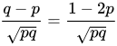
![{\frac {X-\operatorname {E} [X]}{\sqrt {\operatorname {Var} [X]}}}](https://wikimedia.org/api/rest_v1/media/math/render/svg/3bdd3a134128b0517590174937df60485f0828d0)


![{\begin{aligned}\gamma _{1}&=\operatorname {E} \left[\left({\frac {X-\operatorname {E} [X]}{\sqrt {\operatorname {Var} [X]}}}\right)^{3}\right]\\&=p\cdot \left({\frac {q}{\sqrt {pq}}}\right)^{3}+q\cdot \left(-{\frac {p}{\sqrt {pq}}}\right)^{3}\\&={\frac {1}{{\sqrt {pq}}^{3}}}\left(pq^{3}-qp^{3}\right)\\&={\frac {pq}{{\sqrt {pq}}^{3}}}(q^{2}-p^{2})\\&={\frac {(1-p)^{2}-p^{2}}{\sqrt {pq}}}\\&={\frac {1-2p}{\sqrt {pq}}}={\frac {q-p}{\sqrt {pq}}}.\end{aligned}}](https://wikimedia.org/api/rest_v1/media/math/render/svg/3ad7bf226e1980a4b3ed35773624b3e968d61933)
05Higher moments and cumulants
The raw moments are all equal because 

![\operatorname {E} [X^{k}]=\Pr(X{=}1)\cdot 1^{k}+\Pr(X{=}0)\cdot 0^{k}=p\cdot 1+q\cdot 0=p=\operatorname {E} [X].](https://wikimedia.org/api/rest_v1/media/math/render/svg/a40f761815ce1ea63632ed45ef16a5361fa94314)
The central moment of order 

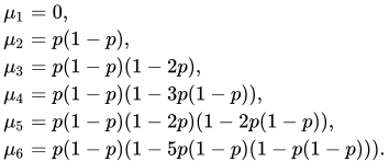


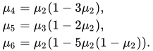
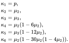
06Entropy and Fisher's Information
Entropy
Entropy is a measure of uncertainty or randomness in a probability distribution. For a Bernoulli random variable 
![{\begin{aligned}H(X)&=\mathbb {E} _{p}\ln {\frac {1}{\Pr(X)}}\\[1ex]&=-\Pr(X{=}0)\ln \Pr(X{=}0)-\Pr(X{=}1)\ln \Pr(X{=}1)\\[1ex]&=-(q\ln q+p\ln p).\end{aligned}}](https://wikimedia.org/api/rest_v1/media/math/render/svg/42ef24eb709e0c06924d709cd77565f43285572c)
The entropy is maximized when 


Fisher's Information
Fisher information measures the amount of information that an observable random variable

Proof:
- The Likelihood Function for a Bernoulli random variable
This represents the probability of observing
- The Log-Likelihood Function is:
- The Score Function (the first derivative of the log-likelihood with respect to
- The second derivative of the log-likelihood function is:
- Fisher information is calculated as the negative expected value of the second derivative of the log-likelihood:


![{\begin{aligned}I(p)=-E\left[{\frac {\partial ^{2}}{\partial p^{2}}}\ln L(p;X)\right]=-\left(-{\frac {p}{p^{2}}}-{\frac {1-p}{(1-p)^{2}}}\right)={\frac {1}{p(1-p)}}={\frac {1}{pq}}\end{aligned}}](https://wikimedia.org/api/rest_v1/media/math/render/svg/930c79a1f00b168593deb05fe32af5d9dcaed143)
It is maximized when
07Related distributions
- If
are independent, identically distributed (i.i.d.) random variables, all Bernoulli trials with success probability p, then their sum is distributed according to a binomial distribution with parameters n and p:
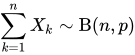 (
(- The Bernoulli distribution is simply
, also written as
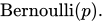
- The categorical distribution is the generalization of the Bernoulli distribution for variables with any constant number of discrete values.
- The Beta distribution is the conjugate prior of the Bernoulli distribution.
- The geometric distribution models the number of independent and identical Bernoulli trials needed to get one success.
- If
, then
has a Rademacher distribution.
Sources and credits
This article is adapted from the Wikipedia article “Bernoulli distribution”, written by its contributors and licensed under CC BY-SA 4.0. Fathomly has changed the layout, removed citation markers, navigation and maintenance notices, and adjusted punctuation. This adapted version is shared under the same license. For references, see the original article.
Images, from Wikimedia Commons:
- Bernoulli Distribution.PNG by Schlurcher, CC BY 4.0
- PMF and CDF of a bernouli distribution.png by Acornellperson, CC0
Fathomly is not affiliated with or endorsed by the Wikimedia Foundation. Spotted a problem? Tell us.
