Bayesian linear regression
Method of statistical analysis
Bayesian linear regression is a type of conditional modeling in which the mean of one variable is described by a linear combination of other variables, with the goal of obtaining the posterior probability of the regression coefficients (as well as other parameters describing the distribution of the regressand) and ultimately allowing the out-of-sample prediction of the regressand (often labelled 

01Model setup
Consider a standard linear regression problem, in which for 


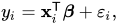
where 

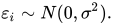
This corresponds to the following likelihood function:

The ordinary least squares solution is used to estimate the coefficient vector using the Moore-Penrose pseudoinverse:

where 


![[y_{1}\;\cdots \;y_{n}]^{\mathsf {T}}](https://wikimedia.org/api/rest_v1/media/math/render/svg/85348072a6ea7c1906d7308c94b8b580121cd58f)
This is a frequentist approach, and it assumes that there are enough measurements to say something meaningful about 
Since the data comprises both 


We can factor out the joint likelihood by assuming strict exogeneity. Strict exogeneity requires:
- that the parameter vector can
be decomposed into two components, with
and
- that data point
not convey any additional information about data point
and the parameter vector

Formally, the first condition requires that 


Under strict exogeneity, the joint likelihood can then be factored into 
02With conjugate priors
Conjugate prior distribution
For an arbitrary prior distribution, there may be no analytical solution for the posterior distribution. In this section, we will consider a so-called conjugate prior for which the posterior distribution can be derived analytically.
A prior 

![{\begin{aligned}(\mathbf {y} -\mathbf {X} {\boldsymbol {\beta }})^{\mathsf {T}}(\mathbf {y} -\mathbf {X} {\boldsymbol {\beta }})&=[(\mathbf {y} -\mathbf {X} {\hat {\boldsymbol {\beta }}})+(\mathbf {X} {\hat {\boldsymbol {\beta }}}-\mathbf {X} {\boldsymbol {\beta }})]^{\mathsf {T}}[(\mathbf {y} -\mathbf {X} {\hat {\boldsymbol {\beta }}})+(\mathbf {X} {\hat {\boldsymbol {\beta }}}-\mathbf {X} {\boldsymbol {\beta }})]\\&=(\mathbf {y} -\mathbf {X} {\hat {\boldsymbol {\beta }}})^{\mathsf {T}}(\mathbf {y} -\mathbf {X} {\hat {\boldsymbol {\beta }}})+({\boldsymbol {\beta }}-{\hat {\boldsymbol {\beta }}})^{\mathsf {T}}(\mathbf {X} ^{\mathsf {T}}\mathbf {X} )({\boldsymbol {\beta }}-{\hat {\boldsymbol {\beta }}})+\underbrace {2(\mathbf {X} {\hat {\boldsymbol {\beta }}}-\mathbf {X} {\boldsymbol {\beta }})^{\mathsf {T}}(\mathbf {y} -\mathbf {X} {\hat {\boldsymbol {\beta }}})} _{=\ 0}\\&=(\mathbf {y} -\mathbf {X} {\hat {\boldsymbol {\beta }}})^{\mathsf {T}}(\mathbf {y} -\mathbf {X} {\hat {\boldsymbol {\beta }}})+({\boldsymbol {\beta }}-{\hat {\boldsymbol {\beta }}})^{\mathsf {T}}(\mathbf {X} ^{\mathsf {T}}\mathbf {X} )({\boldsymbol {\beta }}-{\hat {\boldsymbol {\beta }}})\,.\end{aligned}}](https://wikimedia.org/api/rest_v1/media/math/render/svg/768a22a5f0988a4d25a116f369b5c9b47c3a0400)
The likelihood is now re-written as



This suggests a form for the prior:


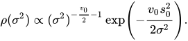
In the notation introduced in the inverse-gamma distribution article, this is the density of an 



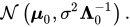
Further the conditional prior density 

In the notation of the normal distribution, the conditional prior distribution is
Posterior distribution
With the prior now specified, the posterior distribution can be expressed as

With some re-arrangement, the posterior can be re-written so that the posterior mean 



To justify that 

Now the posterior can be expressed as a normal distribution times an inverse-gamma distribution:

Therefore, the posterior distribution can be parametrized as follows.

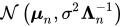



which illustrates Bayesian inference being a compromise between the information contained in the prior and the information contained in the sample.
Model evidence
The model evidence 

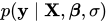



Here 

03Other cases
In general, it may be impossible or impractical to derive the posterior distribution analytically. However, it is possible to approximate the posterior by an approximate Bayesian inference method such as Monte Carlo sampling, INLA or variational Bayes.
The special case 
A similar analysis can be performed for the general case of the multivariate regression and part of this provides for Bayesian estimation of covariance matrices: see Bayesian multivariate linear regression.
Sources and credits
This article is adapted from the Wikipedia article “Bayesian linear regression”, written by its contributors and licensed under CC BY-SA 4.0. Fathomly has changed the layout, removed citation markers, navigation and maintenance notices, and adjusted punctuation. This adapted version is shared under the same license. For references, see the original article.
Fathomly is not affiliated with or endorsed by the Wikimedia Foundation. Spotted a problem? Tell us.